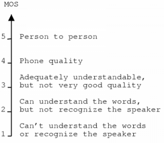
Figure 4.1: Mean Opinion Score (MOS) [23]
In the previous chapter we learned that for one-way voice communication, a bandwidth of 64 kbps is sufficient. For a LAN it is not a problem to achieve this rate, but for dial-up links at this time that rate is not possible. Even a LAN may get quite heavily loaded when VoIP is used in virtual environments, since there could be incoming packets from a large amount of senders at the same time. If we are considering a WAN, it is also not always possible to attain that rate since one slower link is enough to prevent it.
Clearly there is a need for compression and luckily voice information offers the possibility of large compression ratios. In this chapter we will take a look at several compression techniques and explain their importance for VoIP. We will start with some general methods and then we will take a look at some waveform coding and vocoding algorithms. The chapter ends with a discussion about some compression standards for Voice over IP.
We will see in the next chapter that with VoIP usually unreliable protocols are used. It was already mentioned that Voice over IP can tolerate corrupted or lost packets very well, so an unreliable protocol normally does not cause a bad communication quality. Furthermore, reliable protocols rely on the retransmission of packets and these retransmissions add to the overall delay.
An important consequence of the use of unreliable protocols is that compression techniques can only rely on the data in the packet that is to be compressed. Compression algorithms which need information from previous packets cannot be used since it is possible that one of those previous packets did not reach the destination. This would either make decompression impossible or would reconstruct an invalid packet.
One could argue that because of the tolerability of voice communication to errors, this is not a problem. However, with such methods it would mean that one lost or corrupted packet can create several lost packets: all those which relied on the lost packet for compression. So unless the transmission path is highly reliable it is probably better to avoid such compression schemes.
The quality of voice compression is usually measured in terms of Mean Opinion Score (MOS). This is a value between one and five which expresses how close the voice quality is to real-life communication. Figure 4.1 shows this scale.
In this section I will discuss some widely used compression techniques: Lempel-Ziv compression and Huffman coding. These are both lossless compression techniques which means that when data is decompressed, the original data will be restored, without any modifications. This implies that these techniques can be used for both data in general and voice information.
When these methods are directly applied to voice data they do not offer very good compression ratios and for this reason compression is almost never done this way. However, the algorithms can be used as a post-processing step for other compression methods to further enhance the compression ratio, so it is useful to explain them.
Note that several other lossless compression techniques exist. The reason that I will discuss Lempel-Ziv and Huffman compression, is that I have used these schemes in the applications I developed.
There are several Lempel-Ziv (LZ) compression algorithms, but they all work more or less according to the same principles. The algorithms in the LZ family all try to substitute a series of characters by a fixed length code. Two important members of this family are LZ77 and LZ78. An overview of these and other members of the LZ family can be found in [35].
Since I have used the LZ78 algorithm myself, this is the one I will explain. It gives a good idea about the way the LZ algorithms work. The LZ78 algorithm makes use of a `dictionary'. This is a data structure which can hold a number of strings and their length. This dictionary is built both when coding and when decoding. At the start of the algorithm, the dictionary is empty.
The compression algorithm will output doubles <i,c> with `i' being an index into the dictionary and `c' being the next character. At the current position in the data which has to be compressed, the algorithm searches through the dictionary for a match. Suppose a match with length L is found. The current position is then incremented by L. Next, the algorithm outputs a double <i,c> with `i' being the index of the found entry and `c' being the character at the current position. Also, an entry is added to the dictionary. This entry is the concatenation of the found string and the current character. Then the current position is incremented by one and the algorithm again starts searching in the dictionary. The routine is repeated until there is no more data to compress.
If no match is found when searching through the dictionary, the algorithm outputs a double <0,c>. The zero indicates that there was no match and `c' is the character at the current position. The entry which is added to the dictionary contains only the current character. The current position is then incremented by one and the algorithm starts searching the dictionary again.
The decompression algorithm reads doubles <i,c>. If the index `i' is zero, the character `c' is added to the decompression output and an entry containing `c' is added to the dictionary. If `i' is not zero, the concatenation of the dictionary entry at position `i' and the character `c' is made. This new string is added to both the decompression output and the dictionary.
For a given set of possible values and the frequency with which each value occurs, the Huffman algorithm determines a way to encode each value binary. More important, it does this in such a way that an optimal encoding is created. In this section, I will only present the algorithm itself. Proof that it indeed constructs an optimal encoding can be found in [4], which is also the source of the information in this section.
The Huffman algorithm produces a binary string for each value that is to be encoded and these strings can have an arbitrary length. However, the decoding process has to know when a certain binary string has to be replaced by the appropriate value. To be able to do this, the strings must have the following property: none of the binary strings can be a prefix to another string.
Binary strings with this prefix property can be represented by a binary tree in which the branches themselves contain the labels zero and one. The strings which are created by traversing the tree from the root to the leafs are all strings with the prefix property. This is illustrated in figure 4.2.
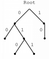
The Huffman algorithm constructs such a tree in which the leafs are marked with the values that need to be encoded. To find out by which binary code a value has to be replaced, you only need to follow the path from the root to the leaf containing that value.
The decompression routine is also easy. The algorithm sets the current position at the root node and starts reading bits. For each bit the appropriate branch is followed. At intermediate nodes the same thing is done, but when a leaf has been reached, the value at that leaf can be output and the current position is reset to the root node. The algorithm then repeats itself.
As you can see, once the tree has been constructed, the algorithm itself is fairly easy. To construct the tree, the algorithm starts with a number of separate nodes, one for each value that needs to be encoded. With each node, the frequency of occurrence of the corresponding value is also associated. For example, if we have got a file in which only the five characters a,b,c,d and e occur with certain frequencies, figure 4.3(a) illustrates a possible situation.
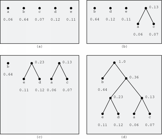
Next, the algorithm looks for the two nodes with the smallest associated frequencies. These two nodes are removed from the list of nodes. A new node is then added to the list and the two removed nodes are its children. The new node's associated frequency is the sum of the frequencies of its children. In the example, the result of this step is depicted in figure 4.3(b).
In this new list of nodes, the algorithm starts it search again for the two nodes with the smallest associated frequencies and the previous step is repeated. In the example, this leads to the situation in figure 4.3(c). When there is only one node left in the list of nodes, this node is the root node of the tree and the algorithm stops. In the example, this leads to the tree in figure 4.3(d).
Waveform coding tries to encode the waveform itself in an efficient way. The signal is stored in such a way that upon decoding, the resulting signal will have the same general shape as the original. Waveform coding techniques apply to audio signals in general and not just to speech as they try to encode every aspect of the signal.
The simplest form of waveform coding is PCM encoding the signal. But a signal can be processed further to reduce the amount of storage needed for the waveform. In general, such techniques are lossy: the decoded data can differ from the original data. Waveform coding techniques usually offer good quality speech requiring a bandwidth of 16 kbps or more.
Differential coding tries to exploit the fact that with audio signals the value of one sample can be somewhat predicted by the values of the previous samples. Given a number of samples, the algorithms in this section will calculate a prediction of the next sampled value. They will then only store the difference between this predicted value and the actual value. This difference is usually not very large and can therefore be stored with fewer bits than the actual sampled value, resulting in compression. Because of the use of a predicted value, differential coding is also referred to as predictive coding.
Differential PCM merely calculates the difference between the predicted and actual values of a PCM signal and uses a fixed number of bits to store this difference. The number of bits used to store this difference determines the maximum slope that the signal can have if errors are to be avoided. If this slope is exceeded, the value of a sample can only be approximated, introducing an amount of error.
In the applications I developed, I have tested a DPCM compression scheme. It used uniformly quantised PCM data as input and produced DPCM output. The predicted value I used was simply the value of the previous sample. Personally, I found that using five bits to store the difference still produced very good speech quality upon decompression. Even with only four bits, the results were quite acceptable.
An extension to DPCM is adaptive DPCM. With this encoding method, there are still a fixed number of bits used to store the difference. In contrast to the previous technique which simply used all of those bits to store the difference, ADPCM uses some of the bits to encode a quantisation level. This way, the resolution of the difference can be adjusted. [26]
Delta modulation can be seen as a very simple form of DPCM. With this method, only one bit is used to encode the difference. One value then indicates an increase of the predicted value with a certain amount, the other indicates a decrease.
A variant of this scheme is called adaptive delta modulation (ADM). Here, the step size used to increase or decrease the predicted value can be adapted. This way, the original signal can be approximated more closely. [10]
With vector quantisation, the input is divided into equally sized pieces which are called vectors. Essential to this type of encoding is the presence of a `codebook', an array of vectors. For each vector of the input, the closest match to a vector in the codebook is looked up. The index of this codebook entry is then used to encode the input vector. [37]
It is important to note that this principle can be applied to a wide variety of data, not only to PCM data. For example, vector quantisation could be used to store an approximation of the error term of other compression techniques.
When we are considering PCM data, we are in fact looking at a signal in the time domain. With transform coding, the signal is transformed to its representation in another domain in which it can be compressed better than in its original form. When the signal is decompressed, an inverse transformation is applied to restore an approximation of the original signal. [37]
One of the domains to which a signal could be transformed is the frequency domain. Using information about human vocal and auditory systems, a compression algorithm can decide which frequency components are most important. Those components can then be encoded with more precision than others. Examples of transformation schemes which are used for this purpose are the Discrete1 Fourier Transform (DFT) and the Discrete Cosine Transform (DCT).
Personally, I have experimented with transform coding using a wavelet transformation. A wavelet decomposition can be used to write a signal as a linear combination of certain wavelet basis functions. The coefficients used in the linear combination then form the wavelet representation of the signal. Using these coefficients for a certain wavelet basis, the original signal can be reconstructed.
A complete explanation of wavelets falls beyond the scope of this thesis. However, the theory of wavelets is very interesting and if you would like more information about it, a good introduction can be found in [44]. This reference is also the source on which I based the implementation of my compression scheme.
The wavelets which I used to transform the signal are called Haar wavelets. They form a very simple wavelet basis. Using these wavelets, decomposition and reconstruction can be done quite fast. They also possess a property called orthonormality which allows us to determine very easily which components of the transformed signal are most important.
In the scheme that I have tried, a uniformly quantised PCM signal was decomposed into its wavelet representation. Next, a number of coefficients with little importance were set zero and the other coefficients were quantised. The resulting sequence of coefficients were then run-length encoded2 and finally, the data was compressed using Huffman coding.
For this last step, I first tried LZ78 compression, but this resulted in little extra compression. Sometimes the resulting code was even larger than before. With Huffman coding, the extra compression was much better. Typically, the code was compressed to sixty to eighty percent of its original size.
Unfortunately, the results are not very spectacular. If good speech quality is to be preserved, this scheme cannot achieve good compression ratios. In fact, I have had better compression results using simple DPCM compression. I believe that this is probably due to the type of wavelets I used.
A typical Haar wavelet is shown in figure 4.4. As you can see, such functions are discontinuous at certain points, which is probably not a desirable property since speech is a relatively slow varying signal. Perhaps other types of wavelets which are more smooth would be more appropriate for speech compression.

Waveform coding methods simply try to model the waveform as closely as possible. But we can exploit the fact that we are using speech information to greatly reduce the required storage space. Vocoding techniques do this by encoding information about how the speech signal was produced by the human vocal system, rather than encoding the waveform itself.
The term vocoding is a combination of `voice' and `coding'. These techniques can produce intelligible communication at very low bit rates, usually below 4.8 kbps. However, the reproduced speech signal often sounds quite synthetic and the speaker is often not recognisable.
To be able to understand how vocoding methods work, a brief explanation of speech production is required.
Figure 4.5 shows the human vocal system. To produce speech, the lungs pump air through the trachea. For some sounds, this stream of air is periodically interrupted by the vocal cords.
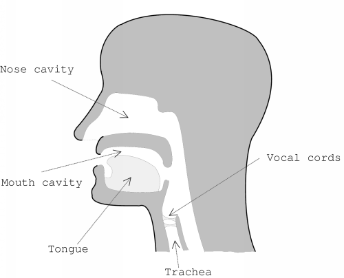
The resulting air flow travels through the so-called vocal tract. The vocal tract extends from the opening in the vocal cords to the mouth. A part of the stream travels through the nose cavity.
The vocal tract has certain resonance characteristics. These characteristics can be altered by varying the shape of the vocal tract, for example by moving the position of the tongue. These resonance characteristics transform the flow of air originating from the vocal cords to create a specific sound. The resonance frequencies are called formants.
Basically, there are three classes of speech sounds that can be produced. Other sounds belong to a mixture of the classes. These are the classes: [33]
An important fact is that the shape of the vocal tract and the type of excitation (the flow of air coming out of the vocal cords) change relatively slowly. This means that for short time intervals, for example 20 ms, the speech production system can be considered to be almost stationary. Another important observation is that speech signals show a high degree of predictability. Sometimes due to the periodic signal created by the vocal cords and also due to the resonance characteristics of the vocal tract. [33]
Instead of trying to encode the waveform itself, vocoding techniques try to determine parameters about how the speech signal was created and use these parameters to encode the signal. To reconstruct the signal, these parameters are fed into a model of the vocal system which outputs a speech signal.
Since the vocal tract and excitation signal change only relatively slowly, the signal that has to be analysed is split into several short pieces. Also, to make analysis somewhat easier, the assumption is made that a sound is either voiced or unvoiced.
A piece of the signal is then examined. If the signal is voiced, the pitch period is determined and accordingly the excitation signal is modelled as a series of periodic pulses. If the speech signal is unvoiced, the excitation will be modelled as noise.
Like we saw in the previous section, the vocal tract has certain resonance characteristics which alter the excitation signal. In vocoders the effect of the vocal tract is recreated through the use of a linear filter.
Perhaps it is not entirely clear what a linear filter is. A filter is any system that takes a signal f(x) as its input and produces a signal g(x) as its output. The output of a filter is also referred to as the response of the filter to a certain input signal. The filter is called a linear filter when scaling and superposition at the input results in scaling and superposition at the output. [11]
A vocoding method will use a specific type of linear filter. The filter will contain certain parameters which have to be determined by the vocoder. This is so because the characteristics of the vocal tract change over time and the coder has to be able to model each state of the vocal tract approximately. Remember that the state of the vocal tract changes only relatively slowly, so for each piece of the input signal, the vocal tract can be considered to have fixed characteristics.
Due to this simple speech production model, speech can be encoded in a very compact way. On the other hand, this simple model is also the cause of the unnatural sounding speech which vocoders often produce.
Several types of vocoders exist, the oldest one being around since even 1939. They all use this simple representation of the speech production system. The main difference between the methods is the vocal tract model used. Below, I will only give a description of the Linear Predictive Coder (LPC) since this vocoder is often discussed in literature about VoIP.
The LPC coder uses the simple model described above. The excitation signal is considered either to be a periodic signal for voiced speech, or noise for unvoiced speech.
The vocal tract model which the LPC method uses, is an approximation of a series of concatenated acoustic tubes [10], as figure 4.6 illustrates.
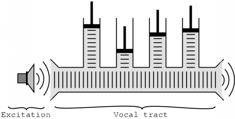
The LPC vocoder examines its input and estimates the parameters to use in the vocal tract filter. It then applies the inverse of this filter to the signal. The result of this is called the residue or residual signal and it basically describes which excitation signal should be used to model the speech signal as closely as possible. From this residual signal, it is relatively easy to determine if the signal is voiced or unvoiced and if necessary, to determine the pitch period.
To determine the parameters for the filter, the LPC algorithm basically determines the formants of the signal. This problem is solved through a difference equation which describes each sample as being a linear combination of the previous ones. Such an equation is called a linear predictor, hence the name of the coder. [24]
The LPC method can produce intelligible speech at 2.4 kbps. The speech does sound quite synthetic however, like with most vocoding techniques.
Waveform coders in general do not perform well at data rates below 16 kbps. Vocoders on the other hand, can produce very low data rates while still allowing intelligible speech. However, the person producing the speech signal often cannot be recognised and the algorithms usually have problems with background noise.
Hybrid coders try to exploit the advantages of both techniques: they encode speech in such a way that results in a low data rate while keeping the speech intelligible and the speaker recognisable. Typical bandwidth requirements lie between 4.8 and 16 kbps.
The hybrid coders that will be discussed in this section are RELP, CELP, MPE and RPE coders. Here, only a brief description is given. A more detailed one can be found in [16], which is the main source for the information in this section.
The basic problem with vocoders is their simplistic representation of the excitation signal: the signal is considered to be either voiced or unvoiced. It is this representation that causes the synthetic sound of these coders. The coders discussed below try to improve the representation of the excitation signal, each in their own way.
The RELP coder works in almost the same way as the LPC coder. To analyse the signal, the parameters for the vocal tract filter are determined and the inverse of the resulting filter is applied to the signal. This gives us the residual signal.
The LPC coder then checked if the signal was voiced or unvoiced and used this to model an excitation signal. In the RELP coder however, the residual is not analysed any further, but will be used directly as the excitation for speech synthesis. The residual is compressed using waveform coding techniques to lower the bandwidth requirements. RELP coders can allow good speech quality at bit rates in the region of 9.6 kbps.
The CELP coder tries to overcome the synthetic sound of vocoders by allowing a wide variety of excitation signals, which are all captured in the CELP codebook. To determine which excitation signal to use, the coder performs an exhaustive search. For each entry in the codebook, the resulting speech signal is synthesised and the entry which created the smallest error is then chosen. The excitation signal is then encoded by the index of the corresponding entry. So basically, the coder uses Vector Quantisation to encode the excitation signal.
This technique is called an analysis-by-synthesis (AbS) technique because it analyses a signal by synthesising several possibilities and choosing the one which caused the least amount of error.
This exhaustive search is computationally very expensive. However, fast algorithms have been developed to be able to perform the search in real-time. CELP techniques allow bit rates of even 4.8 kbps.
Like the previous method, MPE and RPE techniques try to improve the speech quality by giving a better representation of the excitation signal. With MPE, the excitation signal is modelled as a series of pulses, each with its own amplitude. The positions and amplitudes of the pulses are determined by an AbS procedure. The MPE method can produce high quality speech at rates around 9.6 kbps.
The RPE technique works in a similar fashion, only here the pulses are regularly spaced, as the name suggests. The GSM mobile telephone system uses a RPE variant which operates at approximately 13 kbps.
The compression principles discussed above cover pretty much the whole speech compression domain. Due to this fact I was unable to find much information about compression techniques which do not fall into the categories of either waveform coding, vocoding or hybrid coding.
But there is one technique which I find worth mentioning here, namely the use of artificial neural networks for speech compression. At this moment, there is not much information to be found about this particular use of neural networks, but there are documents which describe how neural networks can be used for lossy image compression. It is possible that similar techniques can be used for the compression of speech.
To do this, there are several ways in which artificial neural networks can be used. A neural net could be trained to predict the next sample, give a number of previous samples. This way, the network could perform the predictive function in differential coding schemes. If this prediction is done more accurately than regular predictive techniques this would result in better compression.
Another possible application is to use the neural network in a similar way as a vector quantiser. The network could be trained to map a number of inputs to a specific output. Then, either using a table lookup or another neural network, this number could be used to retrieve an appropriate waveform.
Perhaps a neural network could also be used to perform a speech analysis function which in turn could be used together with some vocoding or hybrid coding technique.
I realise that there is a lot of speculation in this section and unfortunately I did not have the time to conduct experiments using these techniques. However, I strongly believe that neural networks have great potential in a wide variety of applications, including speech compression.
Like we saw in the previous chapter, to be able to preserve good communication quality, the overall delay has to be kept as low as possible. This means that we have to take the delay caused by compression and decompression into account: even if we are able to compress the signal in an excellent way, it has little use for real-time communication if it introduces an unacceptable amount of delay.
Delays during the compression stage can generally be divided into two categories. First of all, there is always some delay due to the calculations which need to be done. This amount of delay depends much on the capabilities of the system performing the compression.
Some compression techniques introduce a second type of delay: to compress a part of the speech signal, they need a portion of the signal which follows the part being handled. The amount of `lookahead' needed determines the amount of delay introduced. For a specific algorithm this delay is fixed and does not vary among systems.
Decompressing the signal can usually be done much faster than compressing it. Of the compression schemes discussed in this chapter, transform coding probably introduces the most delay during decompression since, like during the compression stage, the signal has to undergo a transformation.
With computers becoming ever faster and specialised hardware becoming available, the fixed delay during the compression stage is probably the most important to consider.
To make interoperability between applications possible, it is important that standards are established. The most widely known standards in the VoIP domain, are the G. standards of the ITU-T3. Other well known standards are the ETSI4 GSM standards. Here is a list of some standards: [12]
| Standard | Description | Bit rate | MOS | ||||||||||||||||||||||||||||
|---|---|---|---|---|---|---|---|---|---|---|---|---|---|---|---|---|---|---|---|---|---|---|---|---|---|---|---|---|---|---|---|
| G.711 | Pulse Code Modulation using eight bits per sample, sampling at 8000 Hz | 64 kbps | 4.3 | ||||||||||||||||||||||||||||
| G.723.1 | Dual rate speech coder designed with low bit rate
video telephony in mind [41]. The G.723.1 coder needs
a 7.5 ms lookahead and used one of these coding schemes:
|
Some remarks have to be made at this point. First of all, unfortunately I was not able to find MOS information about some coders. Second, the Mean Opinion Scores are rather subjective and it is probably due to this fact that the MOS values often differ according to different sources. Sometimes these differences are even quite large. For example, in [40] it was mentioned that G.729 annex A had a MOS of 3.4 while [32] claimed that it was 4.0. In this particular case I chose to make a compromise and took the value of 3.7 from [43].
For telephone quality communication using digitised speech, a bandwidth of 64 kbps is needed if the speech data is left uncompressed. But speech data can often be greatly compressed and this can drastically reduce the amount of required bandwidth.
Some compression schemes do not take the nature of the data into account. Such techniques offer some compression, but usually they do not result in high compression ratios. However, they can be used to further reduce the amount of storage needed when another compression technique has already compressed the voice information.
Waveform coding techniques assume that the data is an audio signal, but in general they do not exploit the fact that the signal contains only speech data. They just try to model the waveform as closely as possible. This results in good speech quality at relatively high data rates (16 kbps or above).
Vocoders do exploit the fact that the data is in fact digitised speech. They do not encode the waveform itself, but an approximation of how it was produced by the human vocal system. Such techniques allow very high compression ratios while still providing intelligible communication (at rates of 4.8 kbps or below). However, the reproduced speech usually sounds quite synthetic.
A combination of waveform coding and vocoding techniques is used in hybrid coding schemes. They still rely on a speech production model, but they are able to reproduce the original signal much more closely through the application of waveform coding techniques. These methods can give good speech quality at medium data rates (between 4.8 and 16 kbps).
Compressing and decompressing speech data introduces a certain amount of delay into the communication. Because computers are becoming ever faster and because specialised hardware is becoming available, the amount of lookahead that a compression scheme requires is probably the most important delay component.
To be able to provide interoperability between different applications, it is important that standards are established. Well known compression standards in the VoIP world include the ITU-T's G. series standards and the ETSI's GSM standards.