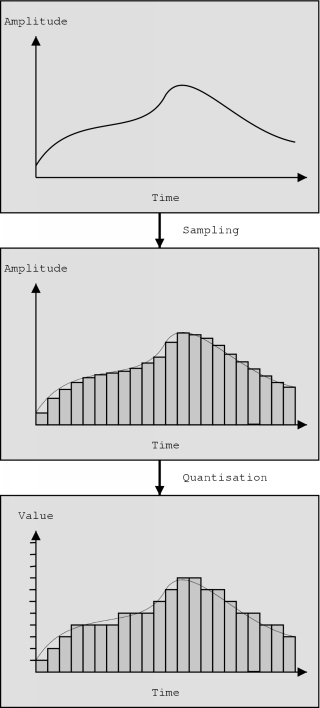
Figure 3.1: Sampling and quantisation
In the previous chapter the Internet Protocol was explained. This was done in a general way, without paying much attention to Voice over IP. Since we now know the most important features of the protocol, we can bring other components of VoIP into the picture.
In this chapter we will take a closer look at some aspects of digitised voice communication. The chapter starts with a discussion about grabbing and reconstruction of voice signals. Next, the requirements for a reasonably good form of voice communication are given. We will then take a closer look at communication patterns and finally we will see what the impact of all these things is on VoIP.
Before you can send voice information over a packet network, you must first digitise the voice signal. After the transmission, the receiver of this digitised signal has to convert it back to an analogue signal, which can be used to generate speaker output. The first stage is also called `grabbing' of the voice signal and the second stage is called reconstruction. In general, these stages are also referred to as analogue-to-digital (A/D) conversion and digital-to-analogue (D/A) conversion, respectively.
As for terminology, it is useful to know that digitising an audio signal is often referred to as pulse code modulation (PCM).
Nowadays, digitisation and reconstruction of voice signals can be done by any PC soundcard, so this is not the most difficult step in creating VoIP applications. For completeness, however, I will give a brief description of the processes.
A continuous signal (a voice signal for example) on a certain time interval has an infinite number of values with infinite precision. To be able to digitally store an approximation of the signal, it is first sampled and then quantised.
When you sample a signal, you take infinite precision measures at regular intervals. The rate at which the samples are taken is called the sampling rate.
The next step is to quantise the sampled signal. This means that the infinite precision values are converted to values which can be stored digitally.
In general, the purpose of quantisation is to represent a sample by an N-bit value. With uniform quantisation, the range of possible values is divided into 2N equally sized segments and with each segment, an N-bit value is associated. The width of such a segment is known as the step size. This representation results in clipping if the sampled value exceeds the range covered by the segments. [10]
With non-uniform quantisation, this step size is not constant. A common case of non-uniform quantisation is logarithmic quantisation. Here, it is not the original input value that is quantised, but in fact the log value of the sample. For audio signals this is particularly useful since humans tend to be more sensitive to changes at lower amplitudes than at high ones [23].
Another non-uniform quantisation method is adaptive quantisation [10]. With such methods, the quantisation step size is dynamically adapted in response to changes in the signal amplitude. PCM techniques which use adaptive quantisation are referred to as adaptive PCM (APCM).
The sampling and (uniform) quantisation steps are depicted in figure 3.1. An important thing to note is that both steps introduce a certain amount of error. It is clear that a higher sampling rate and a smaller quantisation step size will reduce the amount of error in the digitised signal.
Signal reconstruction does the opposite of the digitisation step. An inverse quantisation is applied and from those samples a continuous signal is recreated. How much the reconstructed signal resembles the original signal depends on the sampling rate, the quantisation method and the reconstruction algorithm used. The theory of signal reconstruction is quite extensive and goes beyond the scope of this thesis. A good introduction can be found in [11].
When using VoIP in virtual environments, there is another thing that we must take into account. Each participant will send its own digitised voice signal which will be received by a number of other participants. If two or more persons are talking at the same time, their signals will have to be mixed somehow.
Luckily this is very simple: physics teaches us that for sound waves, the principle of superposition applies. This principle states that when two waves overlap, the amplitude of the combined wave at a specific time can be obtained simply by adding the amplitudes of the two individual waves at that time [38]. Practically speaking this means that we merely have to take the sum of the digitised versions of the signals.
Nowadays everybody is used to telephone quality voice which typically has very few noticeable errors and low delay. Also, when using the telephone system there is no such thing as variation in delay. With packetised voice however, each packet will typically arrive with a slightly different amount of delay, resulting in jitter. There is also no guarantee about delay caused by the network and in general, some packets will contain errors on arrival or will not even arrive at all.
In this section, we will see what the requirements are for decent voice communication. With `decent communication' a form of conversation is meant which does not cause irritation with the participants.
In contrast to data communication, where even the smallest error can cause nasty results, voice communication is much more tolerant to the presence of errors. An occasional error will not seriously disturb the conversation as long as the error does not affect a relatively large portion of the signal.
When you are using data communication, it does not really matter how much delay there is between the sending of a packet and its arrival. With voice communication however, the overall delay is extremely important. The time that passes between one person saying something and another person hearing what was said, should be as low as possible.
Studies show [10] that when the delay exceeds 800 ms, a normal telephone conversation becomes very hard to do. They also show that a delay of 200 to 800 ms is tolerable for short portions of the communication. However, in general a delay below 200 ms has got to be attained to hold a pleasant conversation.
In a conversation between two persons, it it very unlikely that both are always talking at the same time. Usually, when one person is speaking, the other one listens, possibly giving short affirmations. The same principle applies when a group of people is holding a discussion: when one person is talking, the other ones listen.
It is because of this pattern that a normal telephone call wastes a large amount of bandwidth. When someone is not speaking, the bandwidth stays assigned without being used. With packetised voice this bandwidth could be used by other calls or applications.
Several speech models are presented in [10]. Such models could be used to predict arrival patterns of packets containing voice data. These predictions in turn could be used to create a network design with a more effective utilisation of resources. Although these models are obviously important, I feel that they are beyond the scope of this document. If you are interested in these matters, you should refer to [10].
We have just seen some aspects of voice communication. In this section the importance of these aspects for VoIP is described.
At the start of the chapter we saw what sampling and quantisation is. It was also mentioned that a higher sampling rate and a smaller quantisation step implied a better representation of the original signal. But this also means that more digitised information will have to be transmitted and more bandwidth is required. So we have to determine how much information is necessary to hold a telephone quality conversation.
The Nyquist theorem is important in this matter. It states that the minimum sampling frequency should be twice the maximum frequency of the analogue signal [26]. This is in fact quite logical: to be able to capture N cycles, you have to take measures at at least 2N points along the signal. Otherwise it would be impossible to capture the maxima and minima of the signal.
The speech signals that humans produce can contain frequencies of even beyond 12 kHz [10]. However, in the telephone system, only frequencies below 4000 Hz are transmitted and this still allows high-quality communication. Using this information together with the Nyquist theorem suggests that a sampling rate of 8000 Hz is adequate for the digitisation of speech.
To cover the range of amplitudes that a voice signal can produce, at least twelve bits are needed when a uniform quantisation scheme is used [23]. However, a uniform scheme which reduces each sample into an eight bit value is usually good enough to attain telephone quality conversations.
As for logarithmic quantisation, there are two schemes that are also worth mentioning at this point. In the United States and Japan, m-law encoding is the standard for transmission over networks. It reduces a thirteen bit uniformly quantised signal into an eight bit value. In Europe, A-law is used. This scheme does the same but starts with a twelve bit uniformly quantised value. [23]
From this information we can calculate the required bandwidth for a telephone quality conversation. Above was explained that we needed a sampling rate of 8000 Hz and that an eight bit value is usually used to store a sample. So we will be transmitting 8000 eight bit values each second. This requires a bandwidth of at least 64000 bps or 64 kbps.
With Voice over IP, packets can get corrupted or even lost. To reduce the amount of lost information, a packet should contain only a very small amount of the voice signal. This way, if a packet gets lost, only a tiny fraction of the conversation will be missing, which is very unlikely to disturb the conversation.
It is important to note that this argument is made from the point of view of the conversation. We will see later on that from the transmission's point of view, an argument can be made in favour of larger packets. Somehow, a compromise will have to be made.
In a previous section the negative effects of jitter were explained. A simple technique to avoid jitter in the playback of a voice signal, is to introduce an amount of buffering, as figure 3.2 illustrates.
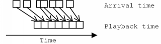
Instead of playing the voice data of an incoming packet as soon as the packet arrives, a small amount of delay is introduced. Because this is done for all packets, there is a higher probability that when one packet has been played, the next one is immediately available.
In practice, normally only a small amount of buffering is needed. In the applications I developed, I have used jitter calculations to determine the amount of buffering needed. The amount of jitter is usually not very high and accordingly only a small amount of buffering is done. This method appears to have good results.
A large delay is disastrous for a conversation. The total delay can be categorised into two types [42]. The first type is fixed delay. This is the total delay which is always present due to buffering, link capacity etc. The second type is variable delay. This is the delay component which is caused by packet queuing in routers, congestions etc.
The components shown in figure 3.3 determine the amount of fixed delay for a VoIP system in virtual environments. For `normal' VoIP, the 3D processing component can simply be left out.
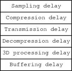
The sampling delay is the delay introduced by the sampling of the voice signal. For example, if the sampling interval is one second, the total delay will be at least one second long since the digitised voice signal cannot be processed before the data is collected. This means that from the point of view of the delay, the sampling interval should be kept as small as possible. Again, from the point of view of the transmission, an argument will be made in favour of larger sampling intervals.
The compression and decompression delays are introduced by compression and decompression algorithms respectively. The transmission delay is the delay which is present due to link capacities. The 3D processing delay is the delay caused by the algorithms which generate the three dimensional sound for use with virtual environments.
Finally, the buffering delay is the delay which is artificially introduced to compensate for jitter. This delay could be set manually or determined automatically, like it is done in my own VoIP applications2.
We saw earlier that in a conversation, there is usually only one person speaking at a time. In packetised voice, this gives us the opportunity to save bandwidth because packets containing only silence do not need to be sent.
However, before we can discard packets, we must first be able to determine whether they contain silence or not. One way this could be done is by calculating the amount of energy of the voice signal in a packet. Packets which do not contain a sufficient amount of energy are assumed to hold only silence and can be discarded.
A simpler technique which I have used is to check a packet for samples with a value above a certain threshold. If no such samples exist, the packet is considered to hold silence and can be discarded. This method has proven to be simple and effective.
Silence suppression does have a minor side effect. Because the `silent' packets are discarded there is absolutely no sound at all at the receiving side, not even background noise. This is truly a deadly silence and it might even seem that the connection has gone. A solution is to artificially introduce some background noise at the receiver side.
Several aspects of voice communication have an important meaning for Voice over IP. To make VoIP possible, we must be able to digitise and reconstruct voice information. A sampling rate of 8000 Hz, using eight bit samples is sufficient to provide telephone quality communication and needs a bandwidth of 64 kbps.
Humans tend to be very tolerant to corrupted or lost voice packets. However, they are far less tolerant to delay and jitter. Jitter should be avoided through the use of buffering as it is disastrous for the quality of the communication. Delay should be kept below 200 ms to maintain a telephone quality conversation.
From the point of view of the communication, small packets are to be preferred since this way, a lost or corrupted packet causes a smaller interruption in the communication. From the delay's point of view, a small sampling interval is important since that interval directly contributes to the overall delay.
Finally, in practice there is usually only one person talking at the same time in a discussion. This means that a lot of bandwidth can be saved by not sending any packets containing only silence. This is called silence suppression.