Background information
Here you can find more information about how the simulation of semiconductor devices is performed. The core equations are called the drift-diffusion equations and are described next. Afterwards, we'll look into how they can be solved on a computer, and how they are used to simulate inorganic or organic solar cells, using a PN-junction model or Metal-Insulator-Metal model respectively.
Drift-diffusion equations
The drift-diffusion equations form a relatively high-level description about what happens to the electrons and holes in an electronic device. In such a model, electrons and holes are not modelled individually, but as a density at each point in the device.
The equations are:
\[ \begin{eqnarray} \vec{\nabla} \cdot \left(\varepsilon_{rel} \vec{\nabla} \phi \right) & = & -\frac{e}{\varepsilon_0}\left(p-n+b\right), \\ \vec{J}_n & = & -D_n \vec{\nabla} n + \mu_n n \vec{\nabla}{\phi}, \\ \vec{J}_p & = & -D_p \vec{\nabla} p - \mu_p p \vec{\nabla}{\phi}, \\ \frac{\partial n}{\partial t} & = & G - R - \vec{\nabla} \cdot \vec{J}_n, \\ \frac{\partial p}{\partial t} & = & G - R - \vec{\nabla} \cdot \vec{J}_p. \end{eqnarray} \]
The first of these equations is Poisson's equation from electrostatics, and specifies the electrostatic potential \(\phi(\vec{r},t)\) that is caused by the distribution of electrons \(n(\vec{r},t)\) and holes \(p(\vec{r},t)\), and possibly a fixed background charge \(b(\vec{r})\). In this version of the equations, \(n\) and \(p\) specify number densities, a certain amount of electrons or holes in a specific region of space, and should of course be positive. While \(b\) is also represented as a number density, its value is allowed to be negative in case the background charge itself is negative. Also in the equation is the relative permittivity \(\varepsilon_{rel}(\vec{r})\) which can take on different values throughout the device but is otherwise fixed, and the vacuum permittivity \(\varepsilon_0\). As usual, \(e\) is the size of the elementary charge.
In the second and third equations, the number currents \(\vec{J}_n\) and \(\vec{J}_p\), for electrons and holes respectively, are calculated. Each number current consists of two contributions: the first term corresponds to the diffusion current which arises as a consequence of concentration differences of electrons or holes between different regions of space. The second part is the drift current and is a result of the response of \(n\) or \(p\) to the electric field \(\vec{E} = -\vec{\nabla}\phi\).
The diffusion constants \(D_n\) and \(D_p\) describe how easily the electrons and holes respond to concentration differences. These values can change thoughout the device, but remain constant in time. The way electrons and holes respond to the electric field is described by the mobilities \(\mu_n\) and \(\mu_p\) of electrons and holes, and are again allowed to vary in space but not in time. Very often the Einstein relation \((D = \mu k T)\) between mobility and diffusion constant is used, so that only one of them will need to be specified.
The equations for the number currents are actually just helper equations, and will need to be inserted in the final two equations. These equations specify how the number currents in combination with generation \(G\) and recombination \(R\) cause the concentrations of electrons and holes to change. The term with the current simply means that if more current is going into a specific region than there's current going out, then the concentration will go up. The generation term \(G(\vec{r})\) specifies the rate at which free electron-hole pairs are generated in the device. While it may vary in space (e.g. if one side of the device is illuminated more than another), it is otherwise kept constant.
In general, the recombination term \(R\) describes the rate at which free electron-hole pairs recombine, causing both the concentrations of \(n\) and \(p\) to go down. Many ways to describe this are possible; the recombination model that we will be using is the relatively simple bimolecular recombination model:
\[ R(\vec{r}, t) = r_f\left(n p - n_i^2 \right) \]
To keep the number of parameters In our simulations limited, the factor \(r_f\) is set to the Langevin prefactor: \[ r_f = e\frac{\mu_n + \mu_p}{\varepsilon_{rel} \varepsilon_0 } \]
The value of \(n_i\) is the intrinsic electron concentration expressed again as a number density.
This set of five drift-diffusion equations describe how the distribution of electrons and holes cause an electrostatic potential, how they respond to potential and concentration differences and how, in combination with generation and recombination of electron-hole pairs, this affects the concentrations of electrons and holes. The variables that can change throughout time are \(n\), \(p\) and \(\phi\), the rest is kept constant (although they may vary in space). The equations shown above actually only describe what goes on in the interior of the device, we still need to specify the behaviour at the boundaries. For our simulations, we use Dirichlet or fixed boundary conditions, meaning that the values of \(n\), \(p\) and \(\phi\) at the boundaries of the simulated device will not change.
In our simulations we will not be interested in the state of the device at any possible time, only the equilibrium or steady state condition will be of interest. In this state, the concentrations of electrons and holes no longer change and the partial derivatives with respect to time in the last two equations will become zero.
Solving the equations
Discretizing the equations
The drift-diffusion equations specified above are a set of partial differential equations, involving continuous changes in position and time. Because we're only interested in the equilibrium situation, the change in time is not very relevant, but the change with respect to position certainly is.
A computer cannot represent continuously changing variables with infinite precision, so we'll have to discretize the equations. In the simulations on these web pages, only a 1D simulation is possible, so let's limit ourselves to this in this explanation. When discretizing such equations, a continuously varying property \(v(x)\), where \(x \in [0, L]\), would be replaced by values \(v_i\) at \(N\) discrete grid points. Here, \(v_1\) corresponds to \(v(0)\) and \(v_N\) to \(v(L)\). The fixed boundary conditions that we're using then imply that \(n_1\), \(n_N\), \(p_1\), \(p_N\), \(\phi_1\) and and \(\phi_N\) are fixed during the simulation, only the contents of \(n_i\), \(p_i\) and \(\phi_i\) for other values of \(i\) will be modified.
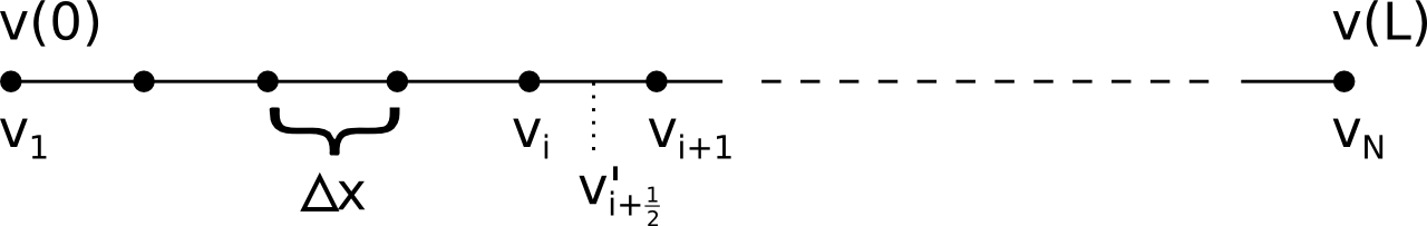
A derivative \(v'(x) = \frac{dv}{dx}(x)\) is then be defined in between grid points, and its value is approximated as \[ v'_{i+\frac{1}{2}} = \frac{v_{i+1} - v_i}{\Delta x} \] where \(\Delta x\) is the distance between grid points, \[ \Delta x = \frac{L}{N-1} \]
While this is the general way the equations are discretized, care must be taken for the equations for the currents. It is possible to use this discretization scheme, but a very large amount of grid points would be needed to obtain accurate results. The reason is that the denstities \(n\) and \(p\) typically vary very rapidly from one point to the next, often in an exponential way.
Much more stable results, even with a low number of grid points (\(\sim\) 100), can be obtained by using the Scharfetter-Gummel method. In this approach, the current is calculated directly for the combined drift and diffusion effects, and is given by: \[ J_{i+\frac{1}{2}} = u\frac{n_i \exp(q) - n_{i+1}}{\exp(q)-1} \] Here, \(u\) is the speed of an electron or hole, based on its mobility and on the electric field: \[ u = \pm \mu \vec{\nabla}\phi = \pm \mu \frac{\phi_{i+1}-\phi_i}{\Delta x} \] where the sign depends on whether we're considering electrons or holes. The value of \(q\) includes the diffusion constant and is defined as: \[ q = \frac{u \Delta x}{D} \]
Time-step based method
General procedure
To look for the steady state solution, the drift-diffusion equations themselves already suggest a way to let the situation evolve towards equilibrium:
- Start with some initial electron and hole number densities \(n\) and \(p\) at each grid point.
- Using these densities, solve Poisson's equation to obtain the corresponding electrostatic potential \(\phi\) at each grid point.
- Calculate the number currents in between the grid points with the Scharfetter-Gummel method described above.
- Combine generation and recombination terms with these number currents to get the rate of change for electron and hole densities \(\frac{\partial n}{\partial t}\) and \(\frac{\partial p}{\partial t}\).
- Multiply these rates with the size of a certain time step \(\Delta t\) and update the corresponding densities.
- Go to step 2.
By repeating this procedure, the simulated device will automatically evolve towards the steady state solution.
In the simulations on the web pages, you need to specify both the size of the time step \(\Delta t\) and the number of times the loop should be repeated. Note that it is up to you to determine an appropriate time step and an appropriate number of steps that should be repeated. When the system has reached equilibrium, the total current througout the device will be the same everywhere, so you can easily tell if you've specified enough time steps.
While a larger value for \(\Delta t\) can make the simulation run faster, a value that is too large will yield unstable behaviour or incorrect results. Because many iterations are typically needed to find the equilibrium situation, this time step based method is usually not very fast. In some cases, an alternative method based on the Newton-Raphson method can find the steady state solution much faster.
Determining the electrostatic potential
In the simulations on the web pages, the value of \(\varepsilon_{rel}\) is not allowed to change from one grid point to the next. While this makes the simulation somewhat less general, it does make it much easier to solve the Poisson equation.
For the 1D simulation that we're considering, in case \(\varepsilon_{rel}\) is the same at every point in space, the discretized version of Poisson's equation becomes: \[ \frac{\phi_{i-1} - 2 \phi_i + \phi_{i+1}}{\Delta x^2} = -e\frac{p_i - n_i + b_i}{\varepsilon_{rel}\varepsilon_0} \] which can be rewritten as \[ -\frac{1}{2} \phi_{i-1} + \phi_i -\frac{1}{2} \phi_{i+1} = e\left(\Delta x^2\right) \frac{p_i-n_i+b_i}{2\varepsilon_{rel}\varepsilon_0} \]
The values of \(\phi\) are fixed at the boundaries, so \(\phi_1\) and \(\phi_N\) will not change. All the equations above for the grid points in between can be written in matrix form as: \[ \left[ \begin{array}{rrrrrrrr} 1 & -\frac{1}{2} & 0 & 0 & 0 & \ldots & 0 & 0 \\ -\frac{1}{2} & 1 & -\frac{1}{2} & 0 & 0 & & 0 & 0 \\ 0 & -\frac{1}{2} & 1 & -\frac{1}{2} & 0 & & 0 & 0 \\ \ldots & & & & & & & \\ 0 & 0 & 0 & 0 & 0 & & -\frac{1}{2} & 1 \\ \end{array} \right] \left[ \begin{array}{l} \phi_2 \\ \phi_3 \\ \phi_4 \\ \ldots \\ \phi_{N-1} \\ \end{array} \right] = \left[ \begin{array}{l} R_2 + \frac{1}{2}\phi_1 \\ R_3 \\ R_4 \\ \ldots \\ R_{N-1} + \frac{1}{2}\phi_{N} \\ \end{array} \right] \] For conciseness, we've introduced the variable \(R_i\) as \[ R_i = e\left(\Delta x^2\right) \frac{p_i-n_i+b_i}{2\varepsilon_{rel}\varepsilon_0} \] Calling the large matrix \(M\), we simply need to determine its inverse to solve Poisson's equation and obtain the values \(\phi_i\) in the interior of the simulated device.
If we call \(N'\) the dimension of the matrix (so \(N'=N-2\), where \(N\) is still the number of grid points), the elements of this inverse matrix are: \[ M^{-1}_{ij} = \frac{2(N'-j+1)i}{N'+1} \quad {\rm if\ } j \ge i \] In case \(j\) is smaller than \(i\), one simply needs to swap their roles, the matrix is symmetric. Multiplying the matrix \(M^{-1}\) with the column vector containing the \(R_i\) values can furthermore be done very efficiently: several intermediate summations can be reused resulting in far less operations than might be suspected at first sight.
In case the value of \(\varepsilon_{rel}\) is allowed to change from one grid point to the next, the matrix \(M\) will still have the same structure (ones on the diagonal with values depending on \(\varepsilon_{rel}\) at the sides), but inverting it and multiplying with the column vector will become more involved.
Newton-Raphson based method
Because we're only interested in the steady state solution of the drift-diffusion equations, we're actually looking for the configuration of \(n\), \(p\) and \(\phi\) for which the following equations hold: \[ \begin{eqnarray} \vec{\nabla} \cdot \left(\varepsilon_{rel} \vec{\nabla} \phi \right) + \frac{e}{\varepsilon_0}\left(p-n+b\right) & = & 0 , \\ G - R - \vec{\nabla} \cdot \vec{J}_n & = & 0 , \\ G - R - \vec{\nabla} \cdot \vec{J}_p & = & 0 . \end{eqnarray} \] These are easily obtained by setting the partial derivatives for the time in the last two equations to zero (because the situation must be the steady state one), and by rearranging Poisson's equation slightly. The expressions for the number currents \(\vec{J}_n\) and \(\vec{J}_p\) are still the same.
Writing the equations in this form illustrates the fact that we're actually looking for a zero-crossing in a multidimensional space; if there are \(N\) grid points, it's the values of \({n_i}\), \({p_i}\) and \({\phi_i}\) that need to be determined, for \(i\) from \(2\) to \(N-2\). We thus have an \((N-2)\times 3\) dimensional space in which we're looking for one particular set of values. Instead of using many time steps to slowly evolve towards the steady state situation, we're now actively looking for only the steady state solution in a direct way. The notion of time has been banned from the equations, we're only looking for one particular state anymore.
A way too look for this multi-dimensional zero crossing, is using the Newton-Raphson method. A straightforward one dimensional example illustrates the basic idea behind this procedure. Suppose one has a curve described by the function \(f(y)\), of which the point \(y\) is sought for which \(f(y) = 0\). The figure below illustrates this - the \(y\) value corresponding to the think black dot is what we're looking for.
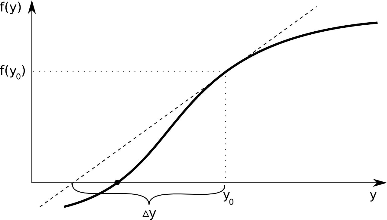
One always starts from an initial guess, let's call this \(y_0\). A first-order Taylor expansion of \(f(y)\) yields the following equation: \[ f(y) \approx f(y_0) + \Delta y \frac{df}{dy}(y_0) \\ \] We know that \(f(y) = 0\) for the point that we're looking for, and if that's true the equation can be rearranged to: \[ \Delta y = - \left(\frac{df}{dy}(y_0)\right)^{-1} f(y_0) \] Of course, our short Taylor expansion is only a very crude approximation, so after adding \(\Delta y\) to our initial guess \(y_0\), most likely we will not have found our correct point \(y\) yet. The basic idea is then to call the new approximation \(y_1\) and repeat the procedure. This results in a sequence of approximations \(y_0\), \(y_1\), \(y_2\), ... which hopefully converges to the correct point.
For the multi-dimensional version, where both the function and the position have an equal number of components, the Taylor expansion for each component of \(F\) (now written as a capital letter to indicate that it can be seen as a column matrix) becomes \[ F^i(Y^1, Y^2, ...) = F^i(Y_0^1, Y_0^2, ...) + \frac{\partial F^i}{\partial Y^j}(Y_0^1, Y_0^2, ...) \Delta Y^j \] or in matrix notation: \[ F(Y) = F(Y_0) + M \Delta Y \] Here, \(Y_0\) is a short notation for \((Y_0^1, Y_0^2, ...)\) and the matrix \(M\) has components \[ M_{ij} = \frac{\partial F^i}{\partial Y^j}(Y_0) \] If one sets \(F(Y)\) to zero, then \(\Delta Y\) becomes: \[ \Delta Y = -M^{-1}F(Y_0) \]
It's easy to imagine situations where things will go wrong or will only converge very slowly to the correct point using this procedure. While there are some things one can do to try to avoid this, especially in a multi dimensional generalization it can become quite tricky to look for the steady state solution in this way.
Having a good starting point is very important when using this method. If this is the case, this method can be much faster than the time step based one, if not, it can just as easily go wrong very fast.
Solving the Newton-Raphson equations using PNaCl
Solving the Netwon-Raphson equations involves inverting a \(3(N-2) \times 3(N-2)\) matrix. While at a first glance this scales very badly with the size \(N\) of the grid, this matrix is actually very sparse which in principle allows for a much faster matrix inversion. When working with simulations in a web page the core programming language one can use is JavaScript, for which unfortunately currently no code exists to invert sparse matrices (as far as we know).
The situation is different if one is not restricted to a web application, but can use a native programming language. In that case, the SuiteSparse library (written in the C programming language) can be used to invert a sparse matrix very efficiently, and this is in fact how it is done in the stand-alone Simiconductor application. In general, such C or C++ code cannot be used directly in a browser. However, the Google Chrome browser supports an extension called Portable Native Client (PNaCl) which allows you to prepare C or C++ code to run in this browser. For this reason, the Newton-Raphson method is only available when using Google Chrome.
Furthermore, because having a good initial guess for the steady state solution is so important when using this method, it will only be used in the calculation of the JV curve. For the first point of the curve, the time step based method will still be used, but for each subsequent point the steady state solution of the previous point will be used as the initial guess for the solution. Since the applied voltage between points typically won't change much, this initial guess is usually a good starting point for the new steady state solution, allowing the Newton-Raphson method to converge quickly to the correct equilibrium situation.
Applied voltage and JV curve
Suppose that we're simulating some kind of solar cell device with the drift-diffusion equations specified above. Consider the case where the device is not illuminated and nothing else is connected to it, so no current can possibly flow. Due to differences in doping (for a PN-junction) or differences in the contacts (for a MIM model), a built-in voltage difference \(V_{bi}\) will arise between the contacts.
When an additional voltage \(V_{app}\) is applied so that current can flow easily, also called forward bias, this means that the total internal voltage drop must be lowered so electrons and holes need less effort in overcoming the potential difference. If the applied voltage makes it more difficult, called reverse bias, the size of the internal voltage drop must increase.
This can all be summarized by the following formula: \[ \Delta \phi = V_{bi} - V_{app} \] Here, \(\Delta \phi\) is the voltage difference (electrostatic potential difference) in the device (so between the end points in our model), \(V_{app}\) is the externally applied voltage and \(V_{bi}\) is the built-in voltage of the device. Using the drift-diffusion equations, one can then calculate the total current of electrons and holes that arises due to a specific applied voltage \(V_{app}\). This yields a curve \(J(V_{app})\) of the total current density in function of the applied voltage, or JV curve for short.
In case there's no illumination, the absence of an applied voltage \(V_{app}\) means that there's only the built-in voltage drop between the end points of the device, which should yield a total current of zero. So without illumination, the JV curve should go through \((0,0)\).
This of course changes when the device is illuminated. When nothing is connected to the device and no current flows, the external voltage difference is no longer zero. Its value is called the open circuit voltage, or \(V_{oc}\). If on the other hand the device contacts are connected by a wire to form a short circuit, the externally applied voltage \(V_{app}\) is zero, but due to the generation of charge carriers there will exist a current. This current is then called the short circuit current (density) \(J_{sc}\).
PN-junction - inorganic solar cell
The drift diffusion equations can be used to simulate a PN-junction. In such a device, a built-in voltage exists, and if one can cause electron-hole pairs to be generated in the region of this built-in electric field, they will be swept away towards the contacts, and an electric current can flow. This is what happens in a inorganic solar cell, where such electron-hole pairs are generated by photons, by incoming light rays.
Effective densities of states
In a semiconductor, the charge transport can be described as happening by electrons present in an energy band called the conduction band, and by holes present in the valence band. The number of electrons in the valence band is determined by the density of states \(g(E)\) and the Fermi distribution function \(f(E)\): \[ n = \int_{E_G}^{\infty} g(E) f(E) dE \]
Here, we assume that the bottom of the conduction band is situated at \(E = E_G\). In a pure semiconductor, this can be approximated as
\[ n = N_C \exp\left(\frac{\mu-E_G}{kT}\right) \]
where
\[ N_C = 2\left(\frac{2\pi m_e kT}{h^2}\right)^{\frac{3}{2}} \]
The value \(N_C\) is the effective number of states (density) in the conduction band, the density of states we can use if we pretend that all of the available energy states are at the bottom of the conduction band. The value \(m_e\) is not simply the rest mass of an electron, it is an effective electron mass, needed to take the actual shape of the energy bands into account, as it differs compared to that of a free electron.
Similarly, we can write for the density of the holes in the valence band (assuming that the top of the valence band is at \(E = 0\)): \[ p = N_V \exp\left(-\frac{\mu}{kT}\right) \] where \[ N_V = 2\left(\frac{2\pi m_h kT}{h^2}\right)^{\frac{3}{2}} \] and \(m_h\) is again an effective mass.
Chemical potential and built-in voltage
In a pure semiconductor, the number of holes always equals the number of electrons. By setting \(n = p\) using the equations above, one can find an approximation of the chemical potential (or Fermi level) \(\mu\):
\[ \mu \approx \frac{1}{2} E_G \]
meaning that for such a material the chemical potential is very close to the center of the band gap.
A pure or intrinsic semiconductor does not conduct electricity well. To improve this, a special way of adding impurities is performed so that additional electrons or holes will be available in the conduction and valence bands respectively. This process is called doping. When one introduces an excess of holes by adding electron acceptors using this process, the resulting material is called a P-type semiconductor; when there's an excess of electrons, by adding electron donors, it's an N-type semiconductor_.
If we consider one particular type of material, adding the extra electrons or holes will cause the chemical potential to change. To determine what the value should be, we can again look at the charge balance. Now, there are not only electrons and holes in the conduction and valence bands, but there are also localized impurities which can be ionized. Overall, the material should be electrically neutral, which we can write as:
\[ n + N_A^{-} = p + N_D^{+} \]
Here, \(N_A^{-}\) is the number of negatively charged acceptors and \(N_D^{+}\) is the number of positively charged donors. Since both can be present in a particular material, both need to be in the equation. Calling \(E_A\) the energy level of the acceptors and calling \(E_G-E_D\) the energy level of the donors (so the donor energy level is \(E_D\) below the conduction band), we can use the Fermi distribution to write \(N_A^{+}\) and \(N_D^{-}\) in terms of the density of acceptors \(N_A\) and donors \(N_D\):
\[ N_A^{-} = N_A f(E_A) \quad {\rm and} \quad N_D^{+} = N_D [1-f(E_G-E_D)] \]
For \(N_D^{+}\) we use the probability that an energy level is occupied by a hole, which is the probability that it is not occupied by an electron, or \(1-f(E)\). Filling this in and rearranging slightly, yields the following equation which needs to be solved for \(\mu\): \[ \exp\left(\frac{\mu-E_G}{kT}\right) + \frac{N_A}{N_C}\frac{1}{\exp\left(\frac{E_A-\mu}{kT}\right)+1} - \frac{N_V}{N_C}\exp\left(-\frac{\mu}{kT}\right) - \frac{N_D}{N_C}\left(1-\frac{1}{\exp\left(\frac{E_G-E_D-\mu}{kT}\right)+1}\right) = 0 \]
Solving the equation - finding \(\mu\)
In the simulation the equation above is solved iteratively. First, we assume that the solution for the chemical potential \(\mu\) will be located inside the gap, so between \(0\) and \(E_G\) in our setup. We define a number of trial values for \(\mu_i\) by distributing them uniformly over the interval: \[ \mu_i = \frac{E_G}{M-1}\times (i-1) \] where M is the number of pieces (chosen to be 16 in the program) and \(i\) goes from \(1\) to \(M\). For each of these \(\mu_i\) values, the left side of the equation is calculated; lets call this \(c(\mu_i)\). There will be some value \(i\) for which \(c(\mu_i) \times c(\mu_{i+1})\) is negative, meaning that that particular interval contains the solution where looking for: if \(c(\mu)\) is negative for one point and positive for another, it must have been zero for some point in between.
If we call these new lower and upper bounds \(\mu_{min}\) and \(\mu_{max}\) respectively, we can create a new series of \(M\) values \(\mu_i\): \[ \mu_i = \mu_{min} + \frac{\mu_{max}-\mu_{min}}{M-1} \times (i-1) \] This will produce a new lower and upper bound for \(\mu\), and we can keep doing this a number of times. This way, a very good approximation to the correct value of \(\mu\) can be found quickly.
Joining P- and N-type materials
In a P-type semiconductor, the chemical potential is lower than for the pure material, while for the N-type version, it is higher. When both materials are present in the same device, the chemical potentials of the two regions align in thermodynamic equilibrium, and a built-in voltage arises.

The size of this built-in voltage is given by the difference in chemical potentials in the two regions: \[ e V_{bi} = \mu_n - \mu_p \]
Simulation boundary conditions
As explained before, the drift-diffusion equations describe what goes on in the interior of the device, but we still need to fix the values of \(n\), \(p\) and \(\phi\) at the boundaries. For the PN-junction model, far away from the contact region between P- and N-type material, the electron and hole concentrations are given by the expressions which use the effective densities of states, using the chemical potential \(\mu_p\) or \(\mu_n\), depending on which region we're in.
This means that for the left-most pixel, the values are fixed at
\[ n_1 = N_C \exp\left(\frac{\mu_p-E_G}{kT}\right) \quad {\rm and} \quad p_1 = N_V \exp\left(-\frac{\mu_p}{kT}\right) \] while for the right-most pixel, these values are: \[ n_N = N_C \exp\left(\frac{\mu_n-E_G}{kT}\right) \quad {\rm and} \quad p_N = N_V \exp\left(-\frac{\mu_n}{kT}\right) \]
For the electrostatic potential, it is only the potential difference that really matters, so for convenience we set the value to zero for the left-most pixel: \[ \phi_1 = 0 \] To get the desired potential difference, the value of the right-most pixel is then set to \[ \phi_N = V_{bi} - V_{app} \] where \(V_{bi}\) is determined from the difference in chemical potentials.
Metal-Insulator-Metal model - organic solar cell
An organic solar cell is often described using a Metal-Insulator-Metal model: the thin layer (e.g. 100 nm) of light absorbing polymer is sandwiched between two metal contacts with different work functions. Unlike in the PN-junction model, where the electrons and holes can be considered as freely moving charges thanks to the organized structure on the atomic level, organic solar cells are very disorganized and in reality charge transport occurs due to 'hopping' from one location to the next.
The energy levels of the electrons can still be considered roughly as being organized in 'bands', with names highest occupied molecular orbital (LUMO) and lowest occupied molecular orbital (HOMO). Insize an organic solar cell, two types of material are present, one which acts as an electron donor, and one as an electron acceptor. In a bulk heterojunction (BHJ) solar cell these two materials are finely mixed, and the resulting device can be modelled similarly as a PN junction. Instead of having a valence band and a conduction band however, one now uses the highest of the HOMO levels as an approximation of the valence band and the lowest of the LUMO levels as the conduction band.
It should be stressed that the underlying physics (transport by hopping) is very different than what is represented by the drift-diffusion equations (freely moving charge carriers). Therefore, it will be more difficult to map the settings of a specific, physical organic solar cell onto the settings needed in the drift-diffusion model.
Built-in voltage
Before bringing the constituents together, the energy diagram of the MIM-model looks like the one on the left in the figure below: at each side of the device, there's a metal contact, with work functions \(C_L\) and \(C_R\) respectively. In between is the organic material (mixture), with the specified effective HOMO and LUMO levels which align well with the work functions of the contacts.
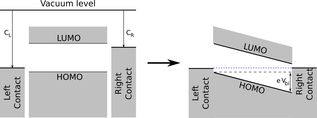
When everything is integrated, in thermodynamic equilibrium the energy levels of the metal contacts will align. This causes an electric field inside the device which, as indicated in the figure, corresponds to a built-in voltage that depends on the work functions of the contacts:
\[ e V_{bi} = C_L - C_R \]
Simulation boundary conditions
Earlier was mentioned that the drift-diffusion equations themselves describe what happens in the interior of the device. To have a consistent set of equations, one still needs to supply boundary conditions for \(n\), \(p\) and \(\phi\). For the MIM-model we use injection barriers at the contacts, where the size of the barrier depends on the difference between contact energy levels and HOMO and LUMO levels.
Calling \(N_{CV}\) the charge carrier density at the contacts, and if we call \(L_u\) the LUMO level and \(H_o\) the HOMO level, the boundary conditions for \(n\) and \(p\) at the left-most pixel become \[ n_1 = N_{CV} \exp\left(-\frac{C_L-L_u}{kT}\right) \quad {\rm and} \quad p_1 = N_{CV} \exp\left(-\frac{H_o-C_L}{kT}\right) \] Similarly, For the right-most pixel one then has: \[ n_N = N_{CV} \exp\left(-\frac{C_R-L_u}{kT}\right) \quad {\rm and} \quad p_N = N_{CV} \exp\left(-\frac{H_o-C_R}{kT}\right) \]
For the electrostatic potential, it is only the potential difference that really matters, so for convenience we set the value to zero for the left-most pixel: \[ \phi_1 = 0 \] To get the desired potential difference, the value of the right-most pixel is then set to \[ \phi_N = V_{bi} - V_{app} \] where \(V_{bi}\) is determined from the difference in chemical potentials.