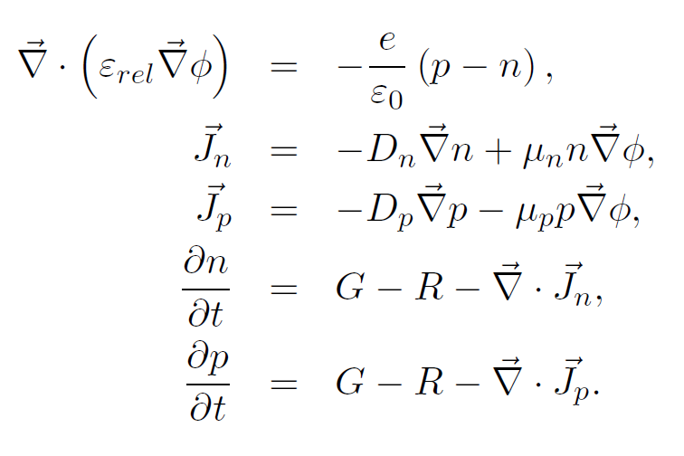
Simiconductor is a program to search for the steady-state solution of the drift-diffusion equations that are shown on the right. These equations were originally used to simulate crystalline semiconductor devices, but are now also used in the study of properties of organic solar cells.
In this model, an electrostatic potential is generated by the distribution of electrons and holes. Gradients in the charge carrier densities and gradients in the this potential then cause currents to be generated, which, in combination with generation and recombination of electron-hole pairs, then caused a change in the charge carrier densities. This process will continue until a dynamic equilibrium has been reached, and neither the charge densities nor the electrostatic potential will change anymore.
The main Simiconductor program is command based, allowing you to configure all parameters of the drift-diffusion equations in the most flexible way. These commands can either be read from a file, or can be entered interactively. In the interactive mode, you can also visualise the defined properties, or see the generated J-V curve. Simulations can be done for either 1D or 2D models, where in the latter case periodic boundary conditions are assumen along one of the axes.
The following document describes in more detail how this main program can be used: simiconductor_eng.pdf
In many cases you will not need or even desire all the flexibility offered by the main program. To make it easier to describe devices in a consistent way, a helper program was created. In this 'region editor', you can define 1D or 2D regions and assign properties to them using a straightforward graphical interface. When this description is complete, you can export these settings to a list of commands that can be read by the main program.
More information about which assumtions are made in this helper program, and how it can be used, can be found in its manual: simiconductor_regioneditor.pdf
Here you can download packages containing both the main Simiconductor program and the region editor for various operating systems; the source code of these programs is available as well. The license which applies to the code is the GPL.
The package: simiconductor-1.1.0.deb
Depends on the packages: libglu1, libqt4-opengl, gsl-bin, python-pyside
The installer: Simiconductor-install.exe
Requires the Visual Studio 2013 redistributable package to be installed.
The installer: Simiconductor-1.1.0.dmg
Requires Qt 4.8 & PySide 1.2 to be installed
The source package: simiconductor-1.1.0.tar.gz
The main program needs the following things installed to be able to build:
The region editor is a Python program which uses PySide for the GUI; it needs:
In this first example, we'll use a device setup for which everything can be calculated analytically. We're going to assume that the electron and hole densities are low, so that they don't influence the electrostatic potential, which then just varies linearly between the values at the contacts. Employing the Einstein relation between diffusion constants and mobilities, and disabling generation and recombination then leads to results from [1]:
where
The JV curve that corresponds to this situation is then
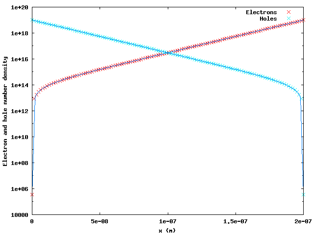 How to set up everything manually, can be seen in the file analytic.txt,
where comments explain what's being done. First, for a specific applied voltage,
an equilibrium situation is calculated. The figure on the right shows the electron
and hole densities obtained by Simiconductor (indicated as crosses) compared to
the analytic results specified above (the blue lines). The correspondence is
clearly very good.
How to set up everything manually, can be seen in the file analytic.txt,
where comments explain what's being done. First, for a specific applied voltage,
an equilibrium situation is calculated. The figure on the right shows the electron
and hole densities obtained by Simiconductor (indicated as crosses) compared to
the analytic results specified above (the blue lines). The correspondence is
clearly very good.
To use this file, you can use the import command: for example, after saving
the analytic.txt file somewhere and starting the Simiconductor program in interactive
mode, you can start typing import and select the downloaded file using the Select file
option in the File menu. The complete path to the file will be inserted in the command
line you're entering, and if you execute the completed import command, the file
will be read and executed.
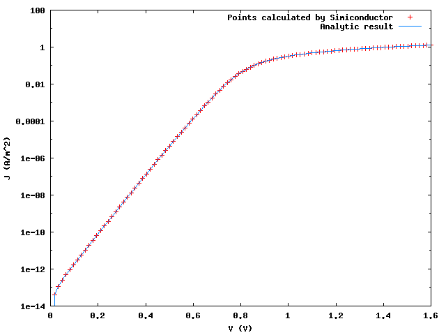 The simulation also calculates a JV curve, and compares the result to the one from the J(V)
relation specified above. Note that the current is represented on a logarithmic scale in this
figure. Here too, the correspondence is clearly very good.
The simulation also calculates a JV curve, and compares the result to the one from the J(V)
relation specified above. Note that the current is represented on a logarithmic scale in this
figure. Here too, the correspondence is clearly very good.
Instead of defining everything manually, we could also create an empty\ image
of 1 pixel by 128 and use this in the region editor. When the properties have
been filled in, the file which will lead to the same simulation can be found in
simple.sit. If this situation is exported to
a file named simple.txt we could use this in the following series of commands
to obtain the exact same JV curve as before:
import simple.txt
sim1/grid/init n
sim1/grid/init p

# Make sure we can start from an equilibrium situation when running
# the sim1/iv command later on
sim1/rundirect

# Now, look for the JV curve. 'VBI' is a value that was defined in
# the file simple.txt
sim1/iv VBI 0 1.6 100 jv2.txt no
In this second example, we'll perform a 1D simulation of a PN-junction. The
commands needed to set up the simulation can be found in pn1d_setup.txt,
which also contains many comments which explain what's being done. To use
this file, save it to disk, start Simiconductor in interactive mode, and
use the import command to read commands from the file, for example:
import pn1d_setup.txt
You'll then see all the commands from the file being executed. This file also
saves the initial situation, in which equilibrium has not yet been reached,
to a file called pn1d_start.dat. This is a binary file, containing the values
that have been set for all grid properties. We can use this to easily load
the created initial situation again.
The movie at the right side shows the evolution of the system towards equilibrium
using the timestep-based method (command name sim1/run). To do this yourself,
you can download pn1d_timestep.txt and
import it again in an interactive Simiconductor session. First, the drift-diffusion
equations are advanced for 300,000 time steps, each corresponding to 1e-16 seconds.
Then we'll do the same number of steps but with a time difference that's ten times
larger. The plots show the current through the device (jx), the hole number density
(p), the electron number density (n) and the electrostatic potential (V).
During the last steps, you'll notice that the current doesn't change anymore,
indicating that equilibrium has been reached. The window with the jx current shows
a curve that looks somewhat strange, but notice that the markers on the Y-axis
show little variation, so this variation is on a very small scale. When the current
is displayed using the sim1/xcur/show command, you'll see that the current at
three locations as well as the overall average current are the same:
simiconductor> sim1/xcur/show
Left average:    -72.9304 A/m^2
Center average:  -72.9304 A/m^2
Right average:   -72.9304 A/m^2
Overall average: -72.9304 A/m^2
Here, we got to the equilibrium situation by using the timestep-based method.
Alternatively, we can also try to obtain the equilibrium situation using the
faster Newton-Raphson method. In this case this also works; the commands you
can use for this can be found in pn1d_direct.txt.
The jx curve will look a bit different, but notice that we're again looking
at it on a very narrow scale. Executing the sim1/xcur/show command again to
show the currents, will produce the exact same results as before.
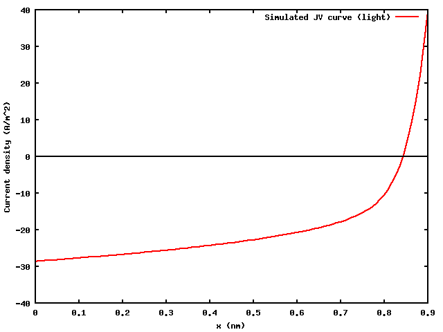 In this example, we're going to recreate the plots from the article [2] by
Koster et al. This is a 1D simulation, which is described in the file
simulation_koster.txt. The file
again contains comments explaining what's going on. The various results
can be plotted using the gnuplot script
createfigures.gnuplot. For example,
the JV-curve that is obtained is shown at the left, and resembles the one
from the article very closely.
In this example, we're going to recreate the plots from the article [2] by
Koster et al. This is a 1D simulation, which is described in the file
simulation_koster.txt. The file
again contains comments explaining what's going on. The various results
can be plotted using the gnuplot script
createfigures.gnuplot. For example,
the JV-curve that is obtained is shown at the left, and resembles the one
from the article very closely.
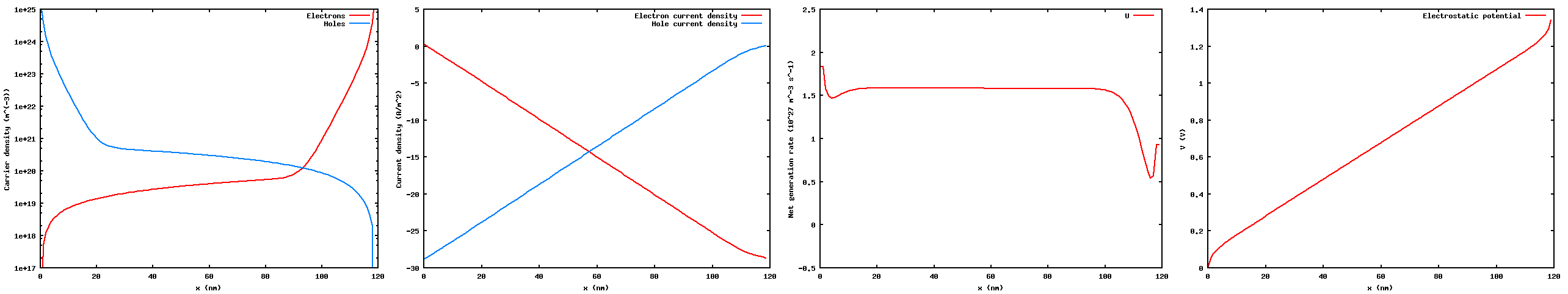
The images below show similar plots as the ones in the article for the open circuit situation. Note that the contacts in our own simulation are reversed with respect to the article. This means that when comparing plots, you'll have to imagine things being mirrored.
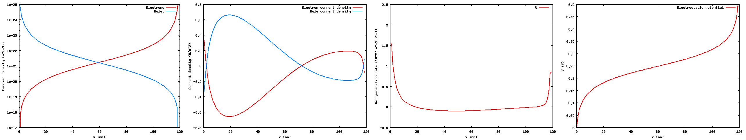
Below, similar plots are shown, but this time they are for the short-circuit situation.
 This example uses a 2D simulation, and mimics one of the simulations described
in [3]. Because it was not entirely clear what parameters are used, the results
will not match as nicely as in the previous example.
This example uses a 2D simulation, and mimics one of the simulations described
in [3]. Because it was not entirely clear what parameters are used, the results
will not match as nicely as in the previous example.
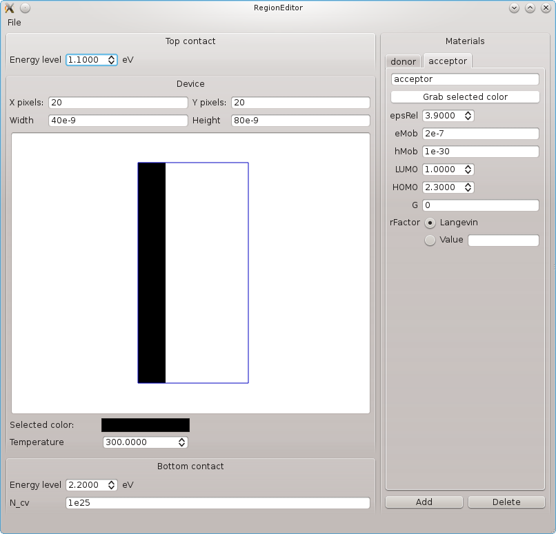
From the article, it appears that the cb1500 simulation was run on a 20x20 grid,
so we're going to use a 20x20 PNG image with the 5:15 ratio of donor to acceptor
material specified as different colors: 20x20px_5_15.png.
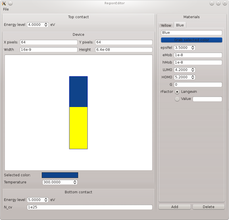
This image is imported into the region editor, and various property values are
entered for the different regions. This results in the situation which can be loaded
from donor_acceptor.sit in the region
editor, and which is also shown on the right.
We can then choose File and Generate 2D to create a file
containing Simiconductor commands that will recreate the situation from the region
editor. Let's call this file donor_acceptor.txt
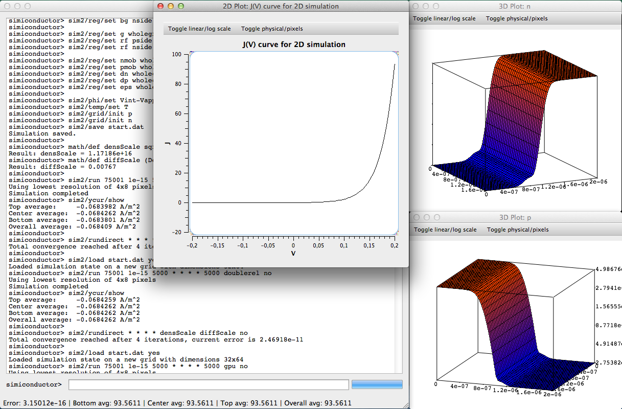
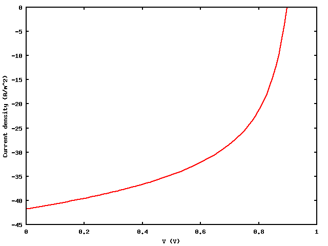 In a file called simulation_donor_acceptor.txt,
the commands from
In a file called simulation_donor_acceptor.txt,
the commands from donor_acceptor.txt can be executed using an import command, after which
we'll run sim2/rundirect to obtain the equilibrium situation. Once this is found,
we start from there to determine the JV curve using the sim2/iv command, the result
of which is shown on the right. This curve resembles the one shown in [3], but as
mentioned before, is does not match exactly.
[1] G. G. Malliaras, J. R. Salem, P. J. Brock and J. C. Scott, Photovoltaic measurement of the built-in potential in organic light emitting diodes and photodiodes, J. Appl. Phys. 84, 1583 (1998)
[2] L. J. A. Koster, E. C. P. Smits, V. D. Mihailetchi and P. W. M. Blom, Device model for the operation of polymer/fullerene bulk heterojunction solar cells, Phys. Rev. B 72, 085205 (2005)
[3] K. Maturová, S. S. van Bavel, M. M. Wienk, R. A. J. Janssen and M. Kemerink, Morphological Device Model for Organic Bulk Heterojunction Solar Cells, Nano Lett., 2009, 9 (8), pp 3032-3037