Tutorial

After following the Installation instructions, you’ll obviously be eager to get started with modeling and inversion of gravitational lens systems. Instead of having to go through all available modules, classes and functions first, this tutorial aims to familiarize you with the core ideas and procedures. You can also take a look at various Example Jupyter notebooks to see them in action immediately.

Modeling and plotting

Modeling gravitational lenses

One of the core parts of the software is the GravitationalLens class. You won’t create an instance of this class directly, that’s prohibited, instead you’ll create a lens model using one of the derived classes, like SISLens for lensing by a Singular Isothermal Sphere, or NFWLens for lensing by a mass distribution with a spherical Navarro-Frenk-White profile. All available models are shown in the documentation of the grale.lenses module; the GravitationalLens class contains the methods that you can call for every one of the the available models. You can also import a LensTool model using the createLensFromLenstoolFile function.

The constructor of a specific lens model always takes two arguments. The first is the angular diameter distance to the lens, the second describes the parameters for the lens model. To convert the redshift of a lens to an angular diameter distance, you can use an instance of the Cosmology class, which destribes a particular cosmological model. Most often, various quantities are expressed in SI units. In grale.constants there are various constants that help you express values in these units, or to convert values to other units.

The following example illustrates the creation of a lens model:

import grale.lenses as lenses
import grale.cosmology as cosmology
from grale.constants import *

# Create a cosmological model with dimensionless Hubble constant h=0.7,
# Omega_m = 0.3 and Omega_lambda = 0.7
cosm = cosmology.Cosmology(0.7, 0.3, 0, 0.7)

# For a lens at z = 0.5, calculate the angular diameter distance
z_d = 0.5
D_d = cosm.getAngularDiameterDistance(z_d)

# Let's show what this angular diameter distance is, in units of Mpc
print("D_d = {:.2f} Mpc".format(D_d/DIST_MPC))

# Create a SIS lens with a velocity dispersion of 250 km/s
sis = lenses.SISLens(D_d, { "velocityDispersion": 250000 })

In this example, we created a single SIS lens, which is centered at the origin. There are many other available models, which are also typically centered at the origin. To make it possible to use a different center, and to even combine multiple lens models into a single, more complex model, we can use a CompositeLens. Continuing from the previous example, we could change the center of the SIS lens, and add a Singular Isothermal Ellipsoid at another location, even rotating it over a specific angle (as the documentation mentions, this angle is interpreted as degrees).

# Create a SIE lens with specific velocity dispersion and ellipticity
sie = lenses.SIELens(D_d, { "velocityDispersion": 200000, "ellipticity": 0.7 })

# Combine these models using a CompositeLens
combLens = lenses.CompositeLens(D_d, [
        { "lens": sis, "factor": 1,
          "x": -1*ANGLE_ARCSEC, "y": -2*ANGLE_ARCSEC, "angle": 0 },
        { "lens": sie, "factor": 1,
          "x": 2*ANGLE_ARCSEC, "y": 1.5*ANGLE_ARCSEC, "angle": 60 }
    ])

You can save save a lens model to a file using the aptly named save function, and load the file again using the load function. The binary data that is loaded or saved, can also be used directly through the fromBytes and toBytes functions. This can help to bypass having to write a lens model to a file first, e.g. when downloading a model from the web, as the following example illustrates by loading the model obtained by inverting CL0024:

import grale.lenses as lenses
import urllib.request

modelUrl = "https://github.com/j0r1/LensModels/blob/master/2008MNRAS.389..415L_CL0024/mainresult_fig2_fig3.lensdata?raw=true"
modelData = urllib.request.urlopen(modelUrl).read()
cl0024Model = lenses.GravitationalLens.fromBytes(modelData)

Plotting lens systems

The plotutil module contains various functions to create plots, using matplotlib, gnuplot or even an interactive 3D plot when using a Jupyter notebook.

Renderers and feedback

By default, calculations will be done on a single CPU core. For a complex lens model, this can become quite slow, and various so called renderers are available to speed up this process. There’s one that can use the different cores on your computer, and even one that can use different computers when the MPI system (e.g. on a supercomputer) is available. For some calculations, OpenCL can use your GPU to speed up calculations, but this is not available for all lens types. To get some feedback during such longer calculations, the feedback module can be useful.

Many of the functions in the plotutil module accept renderer and feedbackObject arguments. While you can specify them in every function used, it will probably be less cumbersome to simply set the default to be used, using setDefaultMassRenderer, setDefaultLensPlaneRenderer and setDefaultFeedback, for example:

import grale.renderers as renderers
import grale.feedback as feedback

# Allowed string values are 'threads' and 'mpi'
renderers.setDefaultMassRenderer("threads")

# Allowed string values are 'threads', 'mpi' and 'opencl'
# (but not all lens models have an OpenCL implementation available)
renderers.setDefaultLensPlaneRenderer("threads")

# Allowed string values are 'none', 'stdout' and 'notebook'
feedback.setDefaultFeedback("notebook")

Single lens plane

In the case of a single lens plane, we can create a plot of the image plane and projected mass density with e.g. the plotImagePlane plotDensity functions. The lens model can be passed as the first argument, which will cause a relevant area to be estimated, which in turn will be used for the plots. In the image plane case, a \(D_{ds}/D_s\) fraction of 1 will be assumed.

To avoid using radians as the unit on the plot axes, we can specify a particular unit to be used with the angularUnit argument of the functions. Alternatively, instead of specifying this argument with every single function, we can also set the default unit using setDefaultAngularUnit function. Note that this only converts values when plotting, it does not change the way function parameters are interpreted for example.

The code below illustrates this, for the combLens model that was created in a previous example:

import grale.plotutil as plotutil
import matplotlib.pyplot as plt

plt.figure(figsize=(10,5))
# Set the unit in which to _display_ plots to one arcsec
plotutil.setDefaultAngularUnit(ANGLE_ARCSEC)

# Create a plot of the image plane for this combined lens
plt.subplot(1,2,1)
plotutil.plotImagePlane(combLens)

# And a plot for the density
plt.subplot(1,2,2)

# This callback will be used to add a color bar
def addBar(a):
    plt.colorbar(a, fraction=0.046, pad=0.04)

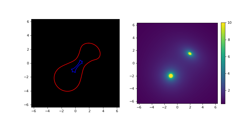
plotutil.plotDensity(combLens, axImgCallback=addBar, vmax=10)
plt.show()

This produces a matplotlib plot containing the two panels shown below, of which the left one shows the image plane (for \(D_{ds}/D_s = 1\)) and the right one shows the density. In the left panel, a red line is used for the critical line and a blue one for the caustic. In the right panel, the vmax argument of the underlying imshow function is used to cut off the color scale at \(10 kg/m^2\) to better show the combination of the circularly symmetric SIS lens and the elliptic SIE lens.

To better control what to plot, e.g. the specific area or source distances, instead of using a lens model as the first argument we can create a LensInfo instance for this situation. Apart from more control about what to plot, this instance will also be used to cache results, so that creating a similar plot may not require everything to be recalculated. This is especially useful as the lens model becomes more complex. When specifying a lens instead of a LensInfo object, internally a LensInfo instance is still generated, and in fact, this instance is typically returned by the functions. So in our previous example we could have obtained this object in the following way:

lensInfo = plotutil.plotImagePlane(combLens)

The following example provides a more extensive example for plotting image plane and mass density information, for the CL0024 lens from an earlier example. In this example, we also set the renderers to threads, so that all available cores on a computer would be used. The plots that are generated by this example are shown below the code (which continues where the CL0024 example left off):

import grale.plotutil as plotutil
import grale.renderers as renderers
import grale.feedback as feedback
import grale.cosmology as cosmology
from grale.constants import *
import matplotlib.pyplot as plt

# Let's create an alias for this class
LI = plotutil.LensInfo

# Set defaults
renderers.setDefaultMassRenderer("threads")
renderers.setDefaultLensPlaneRenderer("threads")
feedback.setDefaultFeedback("stdout")
plotutil.setDefaultAngularUnit(ANGLE_ARCSEC)

# For the generation of this model of CL0024, the
# following cosmology and redshifts were used
cosm = cosmology.Cosmology(0.71, 0.27, 0, 0.73)
zd, zs = 0.395, 1.675
Ds = cosm.getAngularDiameterDistance(zs)
Dds = cosm.getAngularDiameterDistance(zd, zs)

# Inform the LensInfo object that we're interested in a region that's
# 120" wide, with the specified angular diameter distances.
lensInfo = LI(cl0024Model, size=120*ANGLE_ARCSEC, Ds=Ds, Dds=Dds)

try:
    # This is actually mainly for convenience in generating this
    # documentation: at the end of the file we'll save the LensInfo
    # object, which by then contains calculated lens mapping and mass
    # density data, to a file. If this file already exists, we can
    # just use that to obtain the previously calculated data.
    #
    # This makes generating the documentation much less cumbersome,
    # as calculating the lens mapping and mass density map takes several
    # minutes.
    import pickle
    lensInfo = pickle.loads(open("lensinfo.bin", "rb").read())
except Exception as e:
    print(e)


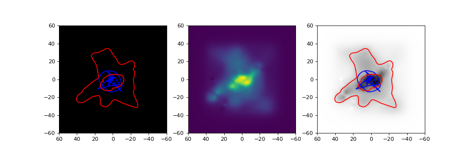
plt.figure(figsize=(12,4))

# Create a plot of the image plane for the cl0024 model. Since the
# right ascension axis goes from right to left, we'll invert the
# X-axis direction.
plt.subplot(1,3,1)
plotutil.plotImagePlane(lensInfo)
plt.gca().invert_xaxis()

# And a plot for the density
plt.subplot(1,3,2)
plotutil.plotDensity(lensInfo)
plt.gca().invert_xaxis()

# Let's also combine the two plots
plt.subplot(1,3,3)
plotutil.plotDensity(lensInfo, cmap="gray_r")
plotutil.plotImagePlane(lensInfo, bgRgb=(0,0,0,0))
plt.gca().invert_xaxis()

plt.show()

# As mentioned before, here we save the generated LensInfo object, to a
# file.
open("lensinfo.bin", "wb").write(pickle.dumps(lensInfo))

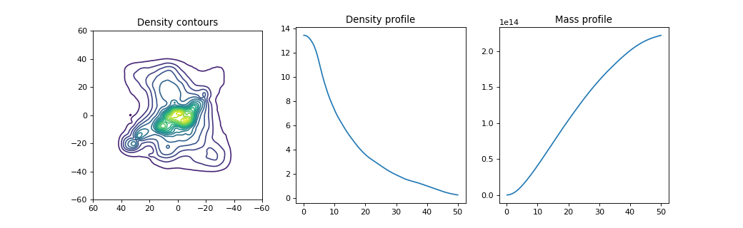
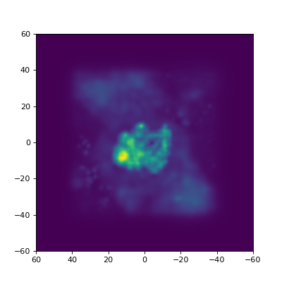
The LensInfo object stores various properties, like the ImagePlane and LensPlane instances that were calculated, as well as the density map. In the example below, we use the plotDensityContours function to create a contour map of the projected mass density of the lens. The result is shown in the panel on the left. The center and right panels of the same figure show the circularly averaged mass density profile and integrated mass profile respectively, using the plotAverageDensityProfile and plotIntegratedMassProfile functions.

plt.figure(figsize=(13,4))
plt.subplot(1,3,1)
plotutil.plotDensityContours(lensInfo, levels=20)
plt.gca().invert_xaxis()
plt.gca().set_title("Density contours")

plt.subplot(1,3,2)
plotutil.plotAverageDensityProfile(lensInfo, 50*ANGLE_ARCSEC)
plt.gca().set_title("Density profile")

plt.subplot(1,3,3)
plotutil.plotIntegratedMassProfile(lensInfo, 50*ANGLE_ARCSEC,
                                   massUnit = MASS_SUN)
plt.gca().set_title("Mass profile")

plt.show()

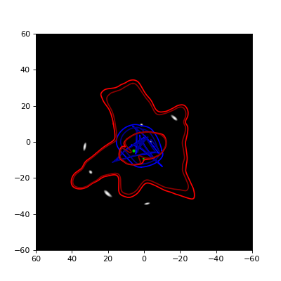
Being able to plot the critical lines and caustics for a lensing scenario is of course nice, but typically we’re also interested in an image configuration that corresponds to a specific source position. For this, we can create a source shape using a class derived from SourceImage, and pass this to e.g. the plotImagePlane function. Note that actually a list of source shapes needs to be specified. The example below illustrates this:

import grale.images as images
import numpy as np

V = lambda x,y: np.array([x,y], dtype=np.double)

src = images.CircularSource(V(5.6,-5)*ANGLE_ARCSEC, 1.1*ANGLE_ARCSEC, fade=True)

plt.figure(figsize=(5,5))
plotutil.plotImagePlane(lensInfo, [src])
plt.gca().invert_xaxis()
plt.show()

You could even create an animation to see what the effect is of different source positions, using Animation or NotebookAnimation. Because the deflection calculations are cached, calculating the lens effect at different source positions or even different source redshifts can be done relatively quickly. The example below is created in the notebook fittest.ipynb, and shows the lens effect of a very strange mass distribution on a circular source.

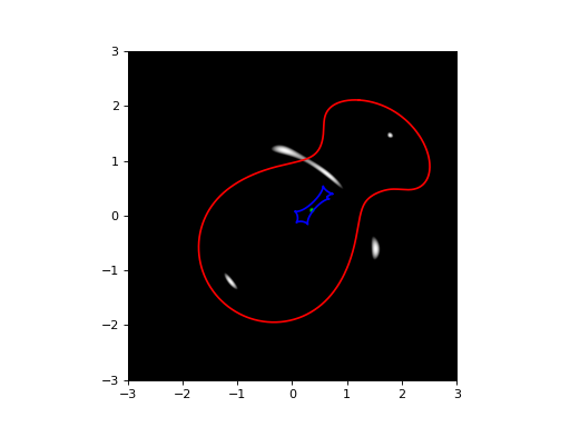
When creating a plot for a single source, or several sources at the same distance/redshift, the last set angular diameter distances (or source redshift) is used. To plot multiple sources, the list of source shapes needs to become a list of dictionaries containing the source shapes as well as the distance information. The code below illustrates this.

# Get distances and shape for a second source
zs2 = 1.3
Ds2 = cosm.getAngularDiameterDistance(zs2)
Dds2 = cosm.getAngularDiameterDistance(zd, zs2)
src2 = images.CircularSource(V(0.21,-9.26)*ANGLE_ARCSEC, 0.75*ANGLE_ARCSEC, fade=True)

# Here, we tell the plotImagePlane function to call 'f' right before
# plotting the image, thereby allowing the pixels to be accumulated
plt.figure(figsize=(5,5))
plotutil.plotImagePlane(lensInfo, [{"shape": src, "Ds": Ds, "Dds": Dds},
                                   {"shape": src2, "Ds": Ds2, "Dds": Dds2}],
                        critColor = [ 'red', 'darkred'],
                        caustColor = [ 'blue', 'darkblue'])

plt.gca().invert_xaxis()
plt.show()

If you don’t just want to plot the mass density of a gravitational lens, but you want to look at the difference between lenses, or even the standard deviation of a whole set of lenses, the DensInfo class can come in handy. It accepts a 2D NumPy array of values, where each value is considered to be the mass density at a specific point. These points are arranged regularly between a bottom-left and top-right corner that also need to be specified. For a specific lens, this kind of information can be obtained using a call to LensInfo.getDensityPoints.

In the example below, we use the CL0024 model again. This is actualy an average of several different individual lens models, and apart from the average mass density associated to the lens, we’re typically also interested in the way these individual models vary. The standard deviation of all these maps can give us some insight into this, and it’s precisely this what is calculated in the example:

import grale.plotutil as plotutil
import grale.renderers as renderers
from grale.constants import *
import numpy as np
import matplotlib.pyplot as plt
import pickle

# Use the available cores for calculating the mass densities, and set the
# plot units to arc seconds
renderers.setDefaultMassRenderer("threads")
plotutil.setDefaultAngularUnit(ANGLE_ARCSEC)

# Create some aliases for these class names
LI = plotutil.LensInfo
DI = plotutil.DensInfo

# The model itself is a CompositeLens, and the parameters will contain
# the individual lens models
params = cl0024Model.getLensParameters()

# We'll store the density maps and the area that's considered in these
# variables.
area, densMaps = None, [ ]

try:
    # This is again a way to speed up the generation of the documentation:
    # if the density maps of the individual lenses have already been 
    # calculated, they can be retrieved from a file
    densMaps, area = pickle.loads(open("densmaps.bin", "rb").read())
except Exception as e:
    print(e)

    # If the density maps don't exist as a file yet, we'll calculate them.
    # For each lens in the CompositeLens, we'll request a calculation of
    # the density points in a certain region. This information is stored
    # so that the standard deviation can be calculated further down.
    for p in params:
        lensInfo = LI(p["lens"], size=120*ANGLE_ARCSEC)
        densMaps.append(lensInfo.getDensityPoints())
        area = lensInfo.getArea()

    # Save the calculated information to a file, to speed up the process
    # of (re-)generating the documentation.
    open("densmaps.bin", "wb").write(pickle.dumps((densMaps,area)))
    
# Calculate the standard deviation of all the individual density maps
# that were calculated
std = np.std(densMaps, 0)

# Create a DensInfo object that links the specified points, containing
# the standard deviation, to a plot area (dictionary with bottom-left and 
# top-right settings)
densInfo = DI(std, **area)

# Plot it in the same way we'd normally plot a GravitationalLens or LensInfo
# object.
plt.figure(figsize=(5,5))
plotutil.plotDensity(densInfo)
plt.gca().invert_xaxis()
plt.show()

Multiple lens planes

Using a LensInfo object, you can also simulate lensing by multiple gravitational lenses as different redshifts. Instead of the LensPlane and ImagePlane classes, internally now MultiLensPlane and MultiImagePlane will be used.

For the lens parameter of the LensInfo object, you now need to specify a list of tuples, where each of the tuples contains a lens model and a redshift. To specify which cosmology must be used to convert the redshifts to angular diameter distances, you can either set the cosmology argument, or install a default cosmological model using setDefaultCosmology The example below illustrates this, more elaborate examples can be found in the Example Jupyter notebooks section.

import grale.images as images
import grale.lenses as lenses
import grale.cosmology as cosmology
import grale.plotutil as plotutil
from grale.constants import *
import numpy as np
import matplotlib.pyplot as plt

# Set a default cosmological model and create an alias for the
# angular diameter function
cosm = cosmology.Cosmology(0.7, 0.3, 0, 0.7)
cosmology.setDefaultCosmology(cosm)
Z = cosm.getAngularDiameterDistance

# Use a default plot unit of one arcsec
plotutil.setDefaultAngularUnit(ANGLE_ARCSEC)

# A shorter name for the LensInfo class
LI = plotutil.LensInfo

# Create a SIS lens with a velocity dispersion of 250 km/s and
# set it at a specific position
z1 = 0.5
sis = lenses.SISLens(Z(z1), { "velocityDispersion": 250000 })
movedSis = lenses.CompositeLens(Z(z1), [
        { "lens": sis, "factor": 1,
          "x": -0.25*ANGLE_ARCSEC, "y": -0.5*ANGLE_ARCSEC, "angle": 0 }
])

# Create a SIE lens with specific velocity dispersion and ellipticity
# at different redshift
z2 = 1.0
sie = lenses.SIELens(Z(z2), { "velocityDispersion": 200000, "ellipticity": 0.7 })
movedSie = lenses.CompositeLens(Z(z2), [
        { "lens": sie, "factor": 1,
          "x": 1*ANGLE_ARCSEC, "y": 0.75*ANGLE_ARCSEC, "angle": 60 }
    ])


# Set the source redshift to 4
zs = 4.0
lensInfo = LI( [(movedSis, z1), (movedSie, z2)], size=6*ANGLE_ARCSEC, zs=zs)

# Create a circular source at a position
V = lambda x,y: np.array([x,y], dtype=np.double)
src = images.CircularSource(V(0.35,0.1)*ANGLE_ARCSEC, 0.05*ANGLE_ARCSEC, 1, True)

# And plot the situation
plotutil.plotImagePlane(lensInfo, [src])
plt.show()

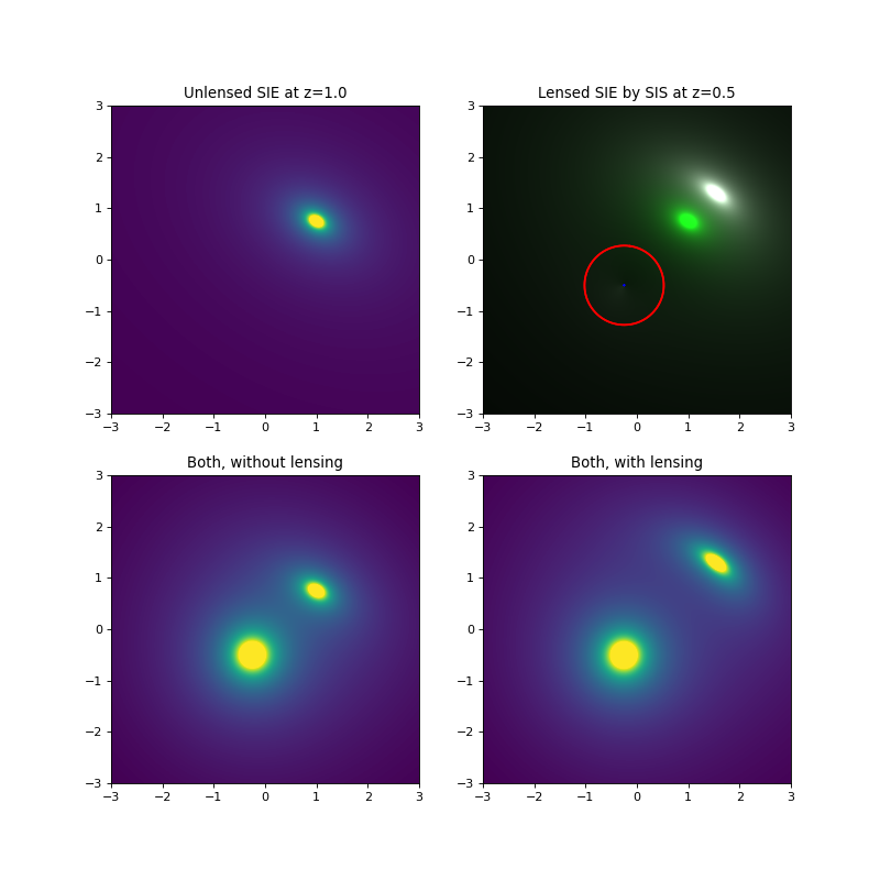
Regarding density plots, this cannot be done when the LensInfo object has been initialized for a multi-lensplane scenario. If you want information about the mass distributions of the individual lenses, you have to obtain the information for the individual lenses, and combine them manually. This way, you can decide yourself whether or not you need to take into account the lens effect of the foreground lens, as is illustrated in the following example, which continues from the SIS and SIE lenses in the previous one:

# A shorter name for the DensInfo class
DI = plotutil.DensInfo

# Create a LensInfo instance for the SIS lens, which we'll use to
# calculate the lens effect on the shape of the SIE
# Here, we specify redshifts instead of angular diameter distances.
lensInfoSIS = LI(movedSis, zd=z1, zs=z2, size=6*ANGLE_ARCSEC)
# For the SIE, we'll only use this to get the shape of the mass
# distribution (as pixels)
lensInfoSIE = LI(movedSie, size=6*ANGLE_ARCSEC)

# Get the densities for both lenses
sisDens = lensInfoSIS.getDensityPixels()
sieDens = lensInfoSIE.getDensityPixels()

# This describes the combination of the densities, without taking the lens
# effect by the foreground SIS into account
comboUnlensed = DI(sieDens + sisDens, **lensInfoSIS.getArea(), isPixels = True)

# To calculate the distortion on the SIE, we'll use its density as a source 
# shape. Because the DiscreteSource expects data in the order of an image (top left
# pixel first), we need to flip it.
sieSrc = images.DiscreteSource(np.flipud(sieDens), 6*ANGLE_ARCSEC, 6*ANGLE_ARCSEC, [0,0])

plt.figure(figsize=(10,10))
plt.subplot(2,2,1)

# First, plot the SIE density itself
plotutil.plotDensity(lensInfoSIE, vmax=10)
plt.gca().set_title("Unlensed SIE at z={}".format(z2))

# We're going to store the lensed image by using this callback as the
# 'processRenderPixels' value. We'll also rescale the brightness a bit, since the
# plotImagePlane routine expects values between 0 and 1. We'll also clip the final
# result, for a cleaner result.
lensedSIE = [ None ]
def f(x):
    if lensedSIE[0] is None:
        # 'x' contains RGB value, which are 3 same values for a gray scale image
        # We're only going to store one of them, to combine it later with the
        # SIS density (which is also a single value per pixel)
        lensedSIE[0] = x[:,:,0].reshape(x.shape[0:2])
    return np.clip(x/10, 0, 1)

plt.subplot(2,2,2)

# First we call the routine without the sources, so we'll only store the lensed
# SIE shape
plotutil.plotImagePlane(lensInfoSIS, [sieSrc], plotSources=False, processRenderPixels = f)

# In the second call, the pixels will no longer be stored in our function
# but the rescaling will still be done.
plotutil.plotImagePlane(lensInfoSIS, [sieSrc], processRenderPixels = f)
plt.gca().set_title("Lensed SIE by SIS at z={}".format(z1))

plt.subplot(2,2,3)
plotutil.plotDensity(comboUnlensed, vmax = 10)
plt.gca().set_title("Both, without lensing")

# Combine the lensed SIE shape with the SIS shape
comboLensed = DI(lensedSIE[0] + sisDens, **lensInfoSIS.getArea(), isPixels = True)
plt.subplot(2,2,4)
plotutil.plotDensity(comboLensed, vmax = 10)
plt.gca().set_title("Both, with lensing")
plt.show()

Modeling arbitrary mass distributions

There are several reasons you might want to be able to calculate the lens effect for a mass distribution of which you don’t know how to expand it in terms of the basic GravitationalLens derived classes: perhaps the lens shape is some analytic model and either the lens effect is not known, or an appropriate model is not available in Grale. Another reason might be that you want to know the lens effect for some pixelized distribution, e.g. the light that’s observed in a cluster and stored in a FITS file.

For the pixelized case, in principle you could use the MultipleSquareLens model and add the effect for each individual pixel. This will certainly work, and depending on the size of the pixels will create a good approximation to the true, non-pixelized distribution. However, the number of pixels will become very large rather quickly, causing the calculations for e.g. the image plane (which itself is subdivided into a large number of locations) to become very slow, even when you can accelerate the calculations by using one of the renderers. Also, the final model will lack some smoothness that may be desired, after all it is built up from square pixels.

To reduce the complexity of the calculation and still obtain a good model, it is possible to create a fit to the mass distribution using Plummer basis functions of varying sizes. To do so, first you create a grid that’s based on the density you’d like to model. Typically, this grid will be created so that the regions that contain more mass will have a more narrow subdivision. Then, using this grid as input, the fitMultiplePlummerLens function is called, which assigns Plummer basis functions to the grid cells (with a width proportional to the cell size), fit the weights of these basis functions to obtain a close match to the target density, and finally returns the result as a MultiplePlummerLens lens model.

The target density needs to be supplied to the fitMultiplePlummerLens function by supplying a callback function. Depending on what you’d like to model, the GridFunction class can be useful, for example to use a FITS file as input with the GridFunction.createFromFITS function.

Examples of this fitting procedure can be found in the fittest.ipynb notebook.

How much the subdivision grid needs to be refined will depend on the complexity of the mass distribution you’re trying to model, and will require some experimentation. In the various createSubdivisionGrid-like functions with which the grid will typically be created, there’s an argument called keepLarger, which defaults to False. In my experience, fitting is somewhat improved by setting this to True; this causes the original grid cell to be present in the subdivision grid even when it’s subdivided further.

Inversion

While creating gravitational lens simulations is interesting in its own right, usually one is far more interested in performing a gravitational lens inversion. Below you can find some information to help get you started, several examples are included in the source code archive to illustrate the procedure.

The origins of the inversion procedure start with 2006MNRAS.367.1209L, but over the years many additions were made, for example to include so-called null-space information (where no images are present), or to include time delay information. A recent overview of the entire procedure can be found in 2020MNRAS.494.3253L.

Overview

You need to specify a few things to be able to start the inversion procedure:

• the observations, usually multiple images of several sources, but could also include e.g. null space data, or weak lensing measurements;

• a set of basis functions (type, location and initial shape/mass) for the lensing mass distribution, of which the weights need to be determined to fit the observations specified as the input.

A genetic algorithm (GA) is then used as the optimization procedure, to look for the weights of these basis functions. The GA looks only for appropriate weights, so e.g. the position or orientation of a basis function will not change.

To be able to model quite arbitrary mass distributions, one typically starts with basis functions (the default type is a Plummer model) laid out in a regular grid pattern. Then, based on a first run of the GA, and therefore a first estimate of the lensing mass distribution, one creates a grid in which cells are subdivided more finely in regions where more mass is detected. This is illustated in the figure below:

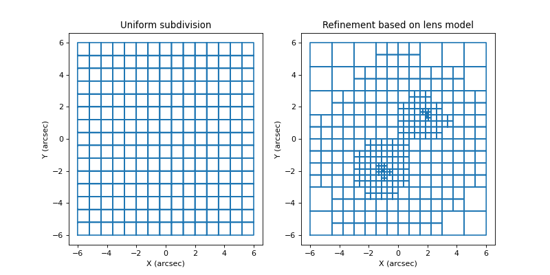
Each cell will again correspond to a basis function of which the weight needs to be optimized, and the GA is executed again to perform this optimization. This subdivision procedure is typically repeated a number of times, with more and more subdivisions/basisfunctions, until the added complexity no longer provides an improvement in the retrieved solution.

Because no particular shape of the mass distribution is assumed, other than the fact that it can be be built up using many simple basis functions, the method is often termed ‘free-form’ or ‘non-parametric’. You could also place specific models, e.g. SIE models, at the location of observed galaxies, and optimize their weights to fit the observations. This is not unlike so-called parametric methods, but note that the GA can only optimize the weights of the basis functions, it cannot alter their location or rotation angle for example.

With an InversionWorkSpace object, it is quite straightforward to execute the needed steps:

• first, you create an InversionWorkSpace where you specify the redshift of the lens, the size of region that will be used for the grid-based procedure, and the center of this region;

• then, you add contraints from observations to the workspace, specified as ImagesData objects;

• you create a grid to lay out the basis functions, either a uniform one, or a subdivision grid based on a previous lens model. Alternatively, you can also manually add basis functions;

• you run the GA to determine the weights of the basis functions, resulting in a mass model.

Based on the resulting mass model, you can create a new grid, start the GA again, etc. This is the main procedure you’ll find in the included examples.

Creating an InversionWorkSpace

In the procedure outlined above, during several refinement steps always the same obvervational input data is used, and typically the same region is used that is subdivided into a number of grid cells. To keep track of these common settings, as well as to perform some other operations, an InversionWorkSpace instance is created.

For example, if a gravitational lens is located at a redshift of 0.4, the strong lensing mass should be retrieved in a 250 arcsec ² region, and a particular cosmological model is to be used, you’d do something like this:

import grale.inversion as inversion
import grale.cosmology as cosmology
from grale.constants import *

z_lens = 0.4
cosm = cosmology.Cosmology(0.7, 0.27, 0, 0.73)
iws = inversion.InversionWorkSpace(z_lens, 250*ANGLE_ARCSEC,
                                   cosmology=cosm)

Instead of specifying the cosmology in the constructor, you could also first set a default one, after which you can just omit the model in the construction of the workspace, i.e. something like:

cosm = cosmology.Cosmology(0.7, 0.27, 0, 0.73)
cosmology.setDefaultCosmology(cosm)

iws = inversion.InversionWorkSpace(z_lens, 250*ANGLE_ARCSEC)

Adding images

Next, we need to specify what the observational constraints are, for example multiply imaged point sources. For such point image data, it is common to have it listed in a text file, and there exists a helper function readInputImagesFile to process such a text file. It returns a list of dictionaries with information about the redshift, the source identifier, and an ImagesData object (describing the actual images), one for each multiply imaged source. Depending on the format of such a text file, it is likely that you need to specify how each line should be analyzed, the documentation lists some examples. If no further processing is required, the call would be something like this:

import grale.images as images

imgList = images.readInputImagesFile("inputpoints.txt", True)

For each image in the list, we then need to call the workspace’s addImageDataToList. In that call, we not only tell the workspace what the relevant redshift is, but also what the type is of the data. In this case the data describes point images, but it could also describe extended images or null space information for example. In our example this would become:

for i in imgList:
   iws.addImageDataToList(i["imgdata"], i["z"], "pointimages")

For extended images it’s also possible to read all the points from a text file, but it’s unlikely that such a file is available. Usually, based on one or more FITS files of the sky region, you can use the GRALE Editor tool to create these data sets, and save them to a file. Again, there would be a different file for each multiply imaged (extended) source. You could load and add these to the workspace like this:

src1 = images.ImagesData.load("source1.imgdata")
src2 = images.ImagesData.load("source2.imgdata")

iws.addImageDataToList(src1, 2.5, "extendedimages")
iws.addImageDataToList(src2, 1.5, "extendedimages")

A null space grid can be created using the helper function createGridTriangles, or you could create it in the GRALE Editor. For point images, the grid is typically a simple grid, but for extended images the irrelevant regions should be cut out (the regions of the images themselves, or a bright cluster galaxy for example).

To allow the inversion algorithm to figure out which null space data belongs to which source, the data must be specified right after the images themselves. For point images, as no holes are cut out there, the same grid can typically be used for each source, and adding the data could become something like this:

bottomLeft = [ -200*ANGLE_ARCSEC, -200*ANGLE_ARCSEC]
topRight = [ 200*ANGLE_ARCSEC, 200*ANGLE_ARCSEC]
nullData = images.createGridTriangles(bottomLeft, topRight, 48, 48)

for i in imgList:
   iws.addImageDataToList(i["imgdata"], i["z"], "pointimages")
   iws.addImageDataToList(nullData, i["z"], "pointnullgrid")

For extended images, as different regions are cut out for different sources, a different file will need to be loaded. The code would then become:

src1 = images.ImagesData.load("source1.imgdata")
null1 = images.ImagesData.load("null1.imgdata")
src2 = images.ImagesData.load("source2.imgdata")
null2 = images.ImagesData.load("null2.imgdata")

iws.addImageDataToList(src1, 2.5, "extendedimages")
iws.addImageDataToList(null1, 2.5, "extendednullgrid")
iws.addImageDataToList(src2, 1.5, "extendedimages")
iws.addImageDataToList(null2, 1.5, "extendednullgrid")

More information about the different types of input data that can be specified this way, can be found in the usage documentation.

Whatever you do, before continuing, make sure that your input data makes sense! Create plots using plotImagesData or load the data in the GRALE Editor.

Creating a grid

As explained before, the usual way to start a lens inversion is to lay out basis functions in a regular grid pattern. In a next step, lens plane basis functions (by default Plummer lenses) will be initialized to have a width that’s proportional to the size of a cell. To set up such a regular grid, use setUniformGrid, for example:

iws.setUniformGrid(15)

This would produce a regular 15x15 grid, with cells that cover the region specified at the workspace’s construction time. As the documentation shows, by default some randomness will be applied to the grid center.

In case you already have a lens model, for example the result from using this uniform grid (let’s call it lens1), you could create a new grid with cells that are finer in regions where there’s more mass. This can be done with a call to setSubdivisionGrid, where you specify a range in which the number of cells should lie. As the 15x15 grid produces 225 cells, in a next step often the range from 300 to 400 is used, for example:

iws.setSubdivisionGrid(lens1, 300, 400)

How many cells exactly this procedure would produce, depends on the mass distribution. In a next iteration, with the optimization result from using this grid, you could for example create a new one as follows:

iws.setSubdivisionGrid(lens2, 500, 600)

The grid that is created this way, can be obtained using InversionWorkSpace.getGrid, and can be visualized easily using plotSubdivisionGrid. This creates plots such as the ones shown above.

Running the inversion

The grid created in the previous step, determines the layout and widths of the basis functions. A call to invert determines the initial masses of these basis functions, and subsequently starts the GA to figure out the weights of the basis functions that are compatible with the observational constraints provided to the workspace. In this invert call, a so called ‘inverter’ can be specified, which allows you to speed up the calculations using e.g. MPI. Alternatively, you can set a default inverter using setDefaultInverter and omit the parameter from the invert call. This would then yield code like the following:

inversion.setDefaultInverter("mpi")
lens1, fitness, fitdesc = iws.invert(512)

The number 512 in the invert call, specifies the number of genomes/chromosomes/individuals in the population of the GA. The function returns the GravitationalLens based lens model that is reconstructed, consisting of the basis functions with weights determined by the GA. This model can be saved and later loaded for further analysis. Apart from this model, the invert call also returns the fitness value that this model had in the GA, together with the type of the fitness measure that was used (e.g extendedimageoverlap or pointimageoverlap depending on the type of the provided input).

To assign initial masses to the basis functions, the mass of the lens is estimated roughly from the provided images. If desired or needed, this can be overridden using the invert call’s massScale argument. The default strategy is to simply divide this mass by the number of grid cells, and assign each grid cell’s basis function that share of the mass. This will automatically place more mass in the more finely subdivided regions. In case you feel this places too much mass in those regions, you can set the rescaleBasisFunctions parameter to True, causing these weights to rescaled according to the size of the cell. In practice, the default setting seems to provide better solutions faster.

Full control over which basis functions are placed where can be obtained by using e.g. addBasisFunctions. This allows you to use any lens model as a basis function. Instead of invert, then the invertBasisFunctions call is required. As a side note, the invert call internally actually calls this function once the basis functions have been derived from the grid.

The massScale parameter also serves another purpose. Each genome in the GA’s population contains the weights of the basis functions for a particular trial solution. As described in the articles, these weights actually only determine the shape of the mass distribution. An overall scale factor will still be searched for, so that the resulting mass distribution yields the best fitness value for that genome. This scale factor will be probed in such a way that the total mass lies in a certain range around massScale. The range can be controlled with the parameter massScaleSearchType.

A special kind of basis function that can be enabled, is a mass sheet basis function. It’s special in the sense that it doesn’t take part in the scaling procedure mentioned above. To enable this, set the sheetSearch parameter to "genome" (the default is "nosheet").

To avoid having to specify the same arguments over and over in the invert calls, you can use setDefaultInversionArguments to set the default values.

In case multiple types of constraints are used, e.g. multiple images as well as null space information, a multi-objective GA will be used. Having multiple constraints, and hence multiple fitness values, implies that there’s in general no longer a single best genome in each generation of the population, but a non-dominated set. The default behavior of the invert call is still to return a single solution based on a priority of the individual fitness measures (can be controlled using the priority parameters, described in the usage documentation). To return the final non-dominated set instead, set the returnNds parameter to True.

Processing the results

The invert call returns a GravitationalLens based lens model, which you can then further analyze as described earlier in the tutorial. For example, you can create plots of the mass distribution, or of the critial lines and caustics.

The workspace’s function backProject can be used to project the images back onto their respective source planes, using a particular lens model (doesn’t even have to be one resulting from the inversion routine). It returns a list of ImagesData instances that have their point coordinates replaced by the back-projected coordinates. Together with the plotImagesData function you could create the plot below, showing the input images as well as the back-projected ones for the first two lens models from the routine outlined previously:

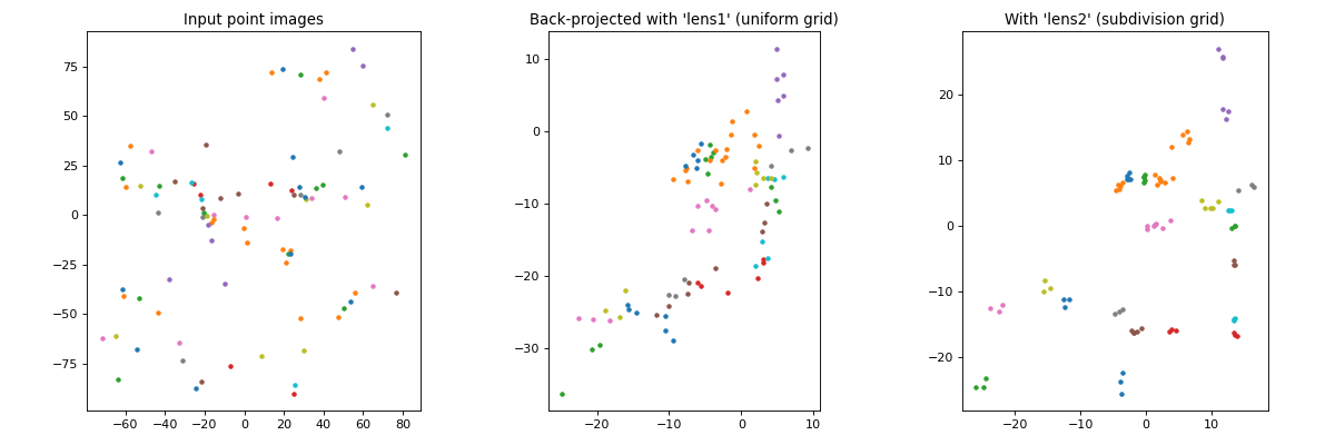
The code to create such a plot looks like this:

bpImgs1 = iws.backProject(lens1)
bpImgs2 = iws.backProject(lens2)

import matplotlib.pyplot as plt

plt.figure(figsize=(15,5))
plt.subplot(1,3,1)
plt.title("Input point images")
plotutil.plotImagesData(imgList)
plt.gca().set_aspect("equal")

plt.subplot(1,3,2)
plt.title("Back-projected with 'lens1' (uniform grid)")
plotutil.plotImagesData(bpImgs1)
plt.gca().set_aspect("equal")

plt.subplot(1,3,3)
plt.title("With 'lens2' (subdivision grid)")
plotutil.plotImagesData(bpImgs2)
plt.gca().set_aspect("equal")

With respect to re-lensing the source estimates, the functions calculateRMS and calculateImagePredictions may be of help. These function reduce each observed image to a single point, which is trivial for point images. In case you’re dealing with extended images, you can control how this needs to be done.

In case you’d like to create a source shape from the backprojected images, the createSourceFromImagesData function may be of interest to you. The source shape this creates is just a simple filled polygon however, in case you’d like to see the actual lens effect using one of the back-projected images as the source, you can calculate this with the GRALE Editor.

You can always calculate the fitness value(s) a specific lens model (again, doesn’t need to be one that resulted from the inversion procedure) has using calculateFitness. For a lens model that was returned using the invert procedure, this should yield roughly the same value as was returned by that function. Not precisely, as the calculateFitness function uses code that’s much different from the optimized code in the inversion routine. The calculations can also take quite some time.

Note on reproducibility

In the procedure that’s outlined above, there are actually two random number generators at work, which is good to know if you’d like to be able to reproduce your results exactly.

The first one is used in the creation of the grid: as mentioned above, by default some randomness is added to the position of the grid center. This randomness comes from Python’s random module, so if you want to make sure that the same grids are generated in different runs, you can set the random number generator’s seed using random.seed. Alternatively, you can save the random number generator’s state using random.getstate which you can then restore if needed using random.setstate.

Instead of working with Python’s random number generator, you can also simply save the generated grids. A grid can be obtained using the workspace’s getGrid function and can be set again using setGrid. To save or load very general Python objects, the easiest way is to pickle/unpickle them.

To perform the inversion, so to run the GA, the Python code will actually start a different program (written in C++), which has its own random number generator. In the output of that program, you’ll see a line like the following, which allows you to find out which seed was used:

GAMESSAGESTR:RNG SEED: 1581199847

To force a specific seed to be used when this inversion program is executed, you can set the GRALE_DEBUG_SEED environment variable. For example, to make sure that seed 12345 is used, one would run the code as follows:

import os
os.environ["GRALE_DEBUG_SEED"] = "12345"
lens1, fitness, fitdesc = iws.invert(512)

Note that with this approach, the same environment variable will still be set for other invert calls as well, which means that the same seed will be used! To reproduce the results from other runs, you’d need to set the seeds those different invert calls used, for example:

os.environ["GRALE_DEBUG_SEED"] = "12345"
lens1, fitness, fitdesc = iws.invert(512)

iws.setSubdivisionGrid(lens1, 300, 400)

os.environ["GRALE_DEBUG_SEED"] = "45678"
lens2, fitness, fitdesc = iws.invert(512)

So, if you create an inversion script and want to be able to reproduce the run exactly, you could print the random number generator’s state at the start, and perform a number of invert calls further on in the script, as follows:

import random
print("RNG State:")
print(random.getstate())

...

iws = inversion.InversionWorkSpace( ... )

...

iws.setUniformGrid(15)
lens1, fitness, fitdesc = iws.invert(512)
lens1.save("inv1.lensdata")

iws.setSubdivisionGrid(lens1, 300, 400)
lens2, fitness, fitdesc = iws.invert(512)
lens2.save("inv2.lensdata")

iws.setSubdivisionGrid(lens2, 500, 600)
lens3, fitness, fitdesc = iws.invert(512)
lens3.save("inv3.lensdata")

To be able to recreate this run exactly, you need to be able to inspect all the output this script generated, so let’s assume you’ve got that in a file somehow. In that file, you can find the random number generator’s state (right below RNG State, which we printed in the script) as well as the seeds that were used in the external inversion program (those GAMESSAGESTR:RNG SEED: lines). Depending on that information, the script to recreate the run would look something like this:

import random
random.setstate((3, (2869744549, 791801109, ... ), None))

...

iws = inversion.InversionWorkSpace( ... )

...

iws.setUniformGrid(15)
os.environ["GRALE_DEBUG_SEED"] = "2551823485"
lens1, fitness, fitdesc = iws.invert(512)
lens1.save("inv1.lensdata")

iws.setSubdivisionGrid(lens1, 300, 400)
os.environ["GRALE_DEBUG_SEED"] = "1662455239"
lens2, fitness, fitdesc = iws.invert(512)
lens2.save("inv2.lensdata")

iws.setSubdivisionGrid(lens2, 500, 600)
os.environ["GRALE_DEBUG_SEED"] = "440472084"
lens3, fitness, fitdesc = iws.invert(512)
lens3.save("inv3.lensdata")

Multi-plane inversion (experimental)

You can also use an InversionWorkSpace object for an inversion involving multiple lens planes. This requires a GPU that provides an OpenCL implementation to perform the multi-plane back-projection of the observed images. This GPU based code at the moment can only calculate the back-projected images, but not time delays or magnifications for example.

Instead of just passing the redshift of a single lens plane, you now pass a list of redshifts, e.g.:

zd1, zd2 = 0.5, 2.0
iws = inversion.InversionWorkSpace([zd1,zd2], 50*ANGLE_ARCSEC)

The same calls to setUniformGrid and setSubdivisionGrid can be used to lay out the basis functions. By default, the functions will be applied to every lens plane, but a particular lens plane can be specified as well.

The result from an invert or invertBasisFunctions call will be a special lens model, of type MultiPlaneContainer, that encapsulated the lens models for the different lens planes. A call to this container’s getLensParameters function will return a list of dictionaries, each with a z entry describing a lens plane’s redshift, and a lens entry that contains the actual lens model for the lens plane at this redshift.

On a technical note, a single GPU is used for one process, which can contain multiple threads. So if you have just a single GPU in your computer, and have eight cores, then setting:

inversion.setDefaultInverter("threads")

Will use that GPU to back-project the images, and use eight CPU threads to calculate the fitness values based on the back-projected points. In case you set:

inversion.setDefaultInverter("mpi")

then the MPI subsystem will start eight different processes, and each of them will try to take control over the GPU. The result of this depends on your GPU. For some, this single GPU can be shared over multiple processes, and it can even run more efficiently than the threads setting. For other GPU’s, access will be restricted to a single process and the initialization will fail.

In case you have multiple GPUs at your disposal, you can use this MPI system to control each of them, and even use multiple threads to process the back-projected images. For instance, suppose that you still have eight cores, but now have two GPUs. You could then specify:

inversion.setDefaultInverter("mpi:2:4")

This means that two MPI processes will get launched, which should be able to use different GPUs. Each of these processes will furthermore use four threads to process the back-projected images.

It is even possible to use GPUs across different nodes in a similar way. After yet another colon, you can add more options for the mpirun command that’s used underneath. Suppose that we now have two such nodes, each with two GPUs and eight cores. With the Intel MPI software, the command would look as follows:

inversion.setDefaultInverter("mpi:4:4:-f /path/to/hostfile -ppn 2")

The first ‘4’ means that four MPI processes will be launched, with two processes per node (-ppn 2), and for which the host names should be in the specified hostfile. Each MPI process will additionally use four threads (the second ‘4’) to calculate the fitness of the back-projected points.

The code will look for an available OpenCL library in some default locations. In case it is not successful in locating the correct library, you can specify the location yourself using the GRALE_OPENCLLIB environment variable.

As mentioned before, the code will automatically try to use different GPUs when available. To coordinate this between different processes, it makes use of a file to which each process can write, and from which each process can read. In some cases it may be necessary to change the name of this file, which can be done using the GRALE_OPENCL_AUTODEVICEFILE environment variable. If multiple PBS or Slurm jobs can end up on the same node, then using the same file name for all jobs will most likely cause problems. In that case, setting a different file name for each job will help, for example something like this in a PBS script:

export GRALE_OPENCL_AUTODEVICEFILE="/dev/shm/grale_gpu_counter_${PBS_JOBID}.dat"

GRALE Editor

The GRALE Editor is a Graphical User Interface (GUI) program to be able to prepare or inspect input files for an inversion, to back-project observed images (from FITS data or an RGB image file), to re-lens a back-projected image and to look for corresponding points in back-projected images.

It is quite similar in concept as the older version, but quite different in design internally, and hopefully easier to use. A major advantage (at least in my view) is the ability to undo (Ctrl-Z, or Cmd-Z on OS X) and redo (Shift-Ctrl-Z, or Shift-Cmd-Z on OS X).

Layers & points

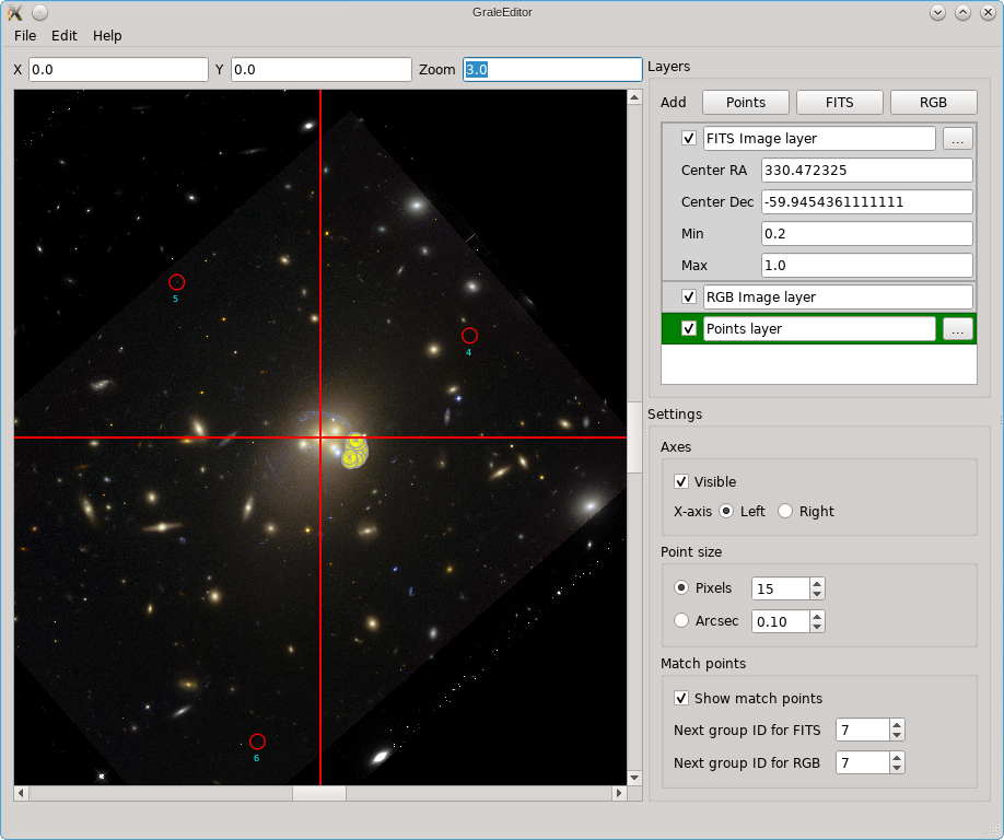
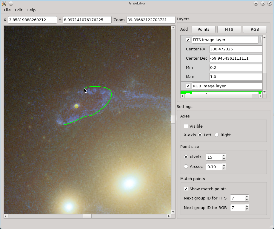
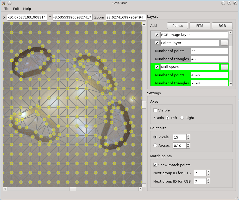
The screenshots below show a number of the core ideas. The main viewport, the left part of each figure, shows a coordinate system on which points can be placed. Near the top of the window, the coordinates (arcsec) corresponding to the mouse pointer’s position are shown, as well as the current zoom. Zooming in/out can easily be done by holding Ctrl/Cmd and using the mouse wheel. To base the coordinates on an actual observation, you can load a FITS file as the background. In the options on the right for this FITS file, you can see that a certain RA/dec coordinate is placed at the center of the coordinate system in the main viewport.

The editor does not provide a way to combine several FITS files from different wavelengths into a color image, but you can import a color image (e.g. a PNG or JPG file) into the editor. You can then match points in the color image to points in the underlying FITS file; that’s what happened in this picture and that’s what those red circles are a remnant of.

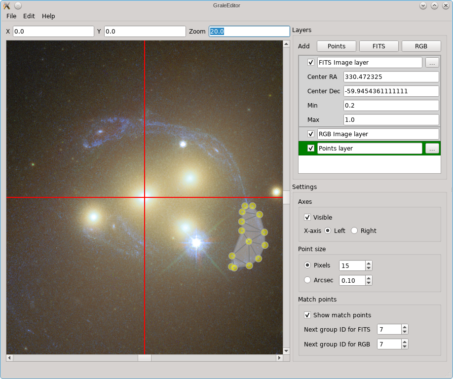
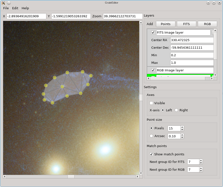
In the picture above, you can also see some yellow dots, although they are not well resolved. After zooming in however you can see that several points as well as a triangulation outline one of the images in Abell 3827.

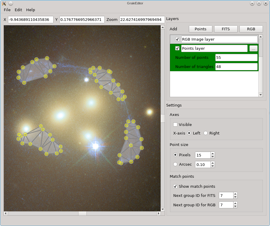
In this example you can see that there are three kinds of layers: for a FITS file, for an RGB image and for points (that can be exported to an ImagesData file). While in this example there is one layer of each, there can be as many as needed, and you can change their order by dragging them around in that ‘Layers’ part of the window. The first layer will be rendered first, that’s why the RGB layer is drawn on top of the FITS layer and hides a big part of the FITS image. With the checkboxes you can control whether or not a layer is shown.

The actions you perform (keyboard/mouse) will have a different effect depending on which layer is active. In the screenshots above, the points layer is the active one, indicated by a dark green color; to change which layer is active, just double click on that layer (I find it easiest to double click just to their left of the checkbox). A left-mouse button click places a point, holding Ctrl/Cmd at the same time will immediately allow you to start typing to add a label/name to the point. To add/change the label later on, just double click on the point. The size of the point and label can be controlled using the option in the right part of the window, where you can opt either to show the point as a fixed number of pixels, or in arcsec units, corresponding to the zoom of the viewport.

For a points layer, this point is a yellow dot, for a FITS layer this is a red cross, and for an RGB layer this is a red circle. The use of the points in FITS/RGB layers, is to be able to mark corresponding points in these layers by giving them the same label. To make this procedure somewhat easier, a label (a number) will be added automatically to these points, based on the ‘Next group ID’ settings on the right. You can always change the label if desired, of course.

Background FITS & matched RGB

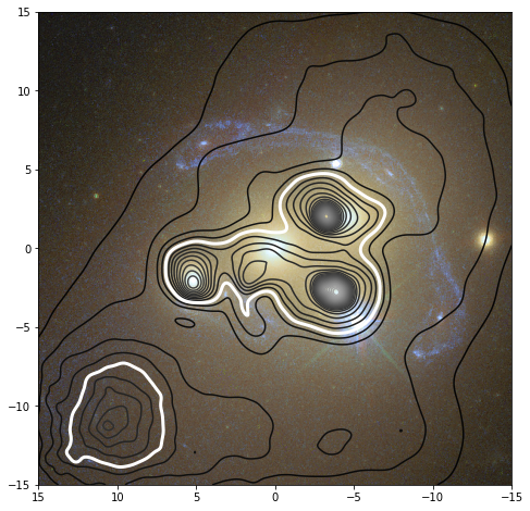
To create such a background FITS and matching RGB image, you start by adding a FITS layer. To specify which point in the FITS image corresponds to the center of the coordinate system, you can double click on that point. Alternatively, you can simply enter the RA/dec coordinates in the layer’s info; by default they have been set to the central pixel’s coordinates.

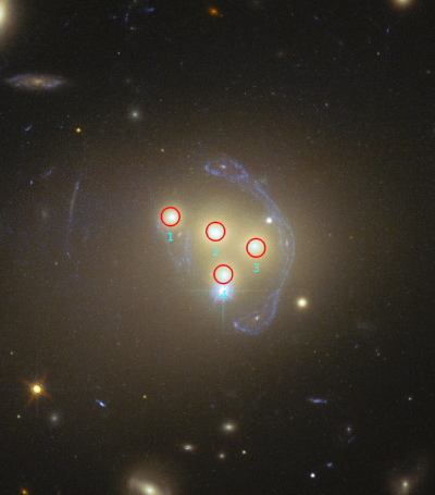
When this layer is active, and you perform a single left mouse click, a red cross will be added with a label that’s specified in the bottom-left of the user interface (‘Next group ID for FITS’). The screenshot below shows the viewport where four such points have been added, roughly at the center of four prominent galaxies.

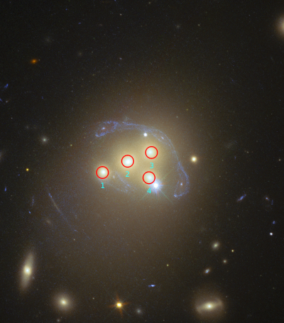
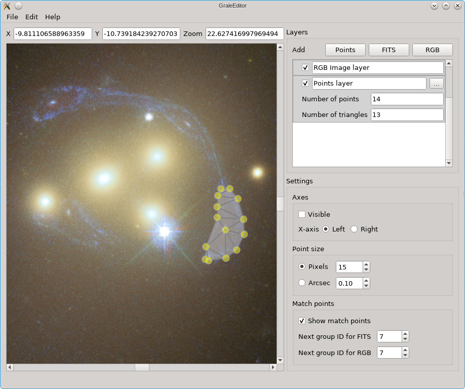
To align an RGB image to this FITS file, first we need to add a new RGB layer, containing e.g. a PNG or JPG file. Initially, the image will just be shown centered in the viewport, will not be aligned yet with the FITS file, even having a different scale. To be able to calculate the necessary transformation, we need to select the same galaxies, which will be shown as red circles. For the example we’re using, this looks something like the image below.

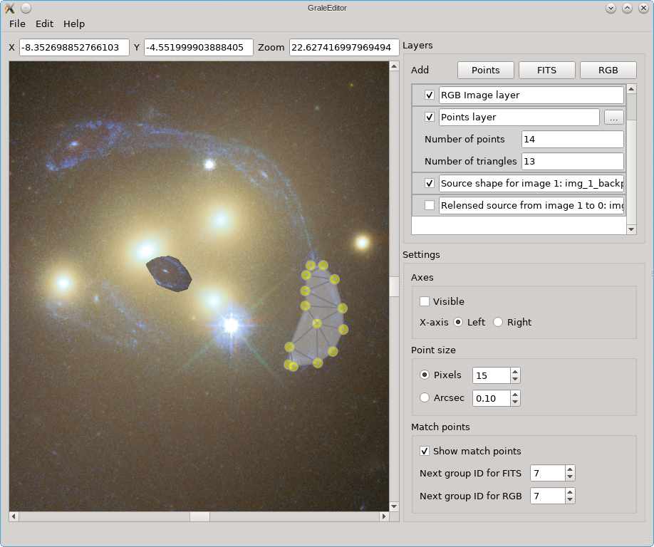
To be able to match the RGB layer to the FITS layer, it’s imperative that the corresponding points have the same label. For a first alignment, it’s not that important that the exact positions match, for now we just want the alignment to be roughly ok. To perform the necessary calculations and align the RGB layer to the FITS layer, just make sure that the RGB layer is active and double click in the main viewport (doesn’t matter where you click). In our example, this yields the following:

To see how well the alignment worked, you can just hide/show the RGB layer so that you can compare it to the underlying FITS image. Since we only roughly selected those galaxies, the alignment will not be that good yet. To get a better alignment, we need to get those points to point to corresponding positions more accurately. To move a point, you can just drag it.

My approach is usually to just forget about those initial points, and add new ones that lie near the borders of the images. Furthermore, to make it easier to pin-point a feature in the FITS/RGB files, I typically look for some very small galaxies that are visible in both images. To delete points, first select them: a single point is selected by clicking on it, by holding Ctrl/Cmd you can add points to the selection, and by holding Shift you can select a range. Pressing Shift+Delete then removes the selected points. With the new matching points, make sure that the RGB layer is active, and double click again to re-calculate the alignment.

Extended images & null space

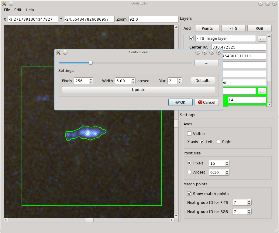
While double clicking on a FITS or RGB layer is related to the background images, double clicking on a point in the viewport when a points layer is active, starts the contour finder tool. In the example below, a left double click on the blueish galaxy was performed (with a points layer being active). The slider then allows you to select a specific contour, indicated by a curved green line. By default, the dialog box is actually a bit smaller, but if you press the three dots ... next to the slider, you’ll see various options that are related to how the contours are determined.

The square region that will be used for the contour finder, is indicated by the green box, the width of which can be set using the aptly named Width parameter. For this region, internally a square gray scale image is generated, subdivided in the specified number of pixels both horizontally and vertically. This internal image is blurred using the specified width, and in the resulting blurred/smoothed image contours are determined. Note that all these operations happen on the image as it is shown, irrespective of whether that’s a FITS layer, an RGB layer or an overlap. If it’s a FITS layer of which the min/max parameters are set in such a way that everything is shown as white for example, then no meaningful contours will be detected. The tool works with how the viewport is shown.

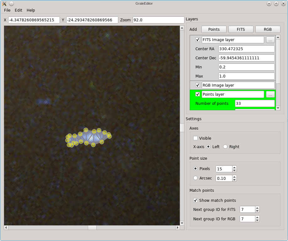
If you press Ok, then the selected contour will be traced with a number of points and these will be triangulated. The resulting points and triangles will be added to the active points layer. The screenshot below shows an example. If there would already be points inside the contour, in the active layer, then these will be included in determining the triangulation.

If the contour tool does not work well enough, you can always simply draw the contour yourself. Just hold the left mouse button and move the mouse pointer to start drawing. The screenshot below illustrates this:

When you release the mouse button, points are added according to the contour that was drawn, and a triangulation is provided. All points and triangles are added to the active points layer. As can be seen in the example below, if a point in the active layer is internal to the contour, it is used in the triangulation.

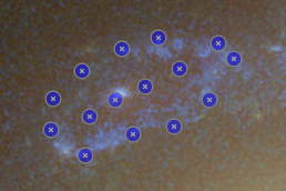
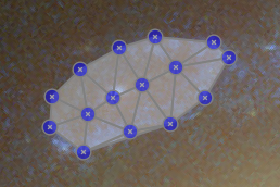
You can also follow a completely manual approach: first just add individual points using a single left click each time. Then, select the points for which you’d like to add a triangulation. To select points, you can select an entire region by keeping the Shift key pressed, holding down the left mouse button and select a rectangular range. Alternatively, you can select multiple points individually by keeping Ctrl (or Cmd on OS X) pressed down, and clicking on the existing points individually. In either case, a selected point will turn blue instead of yellow. The figure on the left shown this. To create a triangulation from these points, just double click on one of the selected points. This in turn would produce the situation on the right.

To delete points or triangles, first select them as before. Then, to delete both points and triangles press Shift+Delete. To only delete the selected triangles but not points that could be selected as well, press Ctrl+Delete.

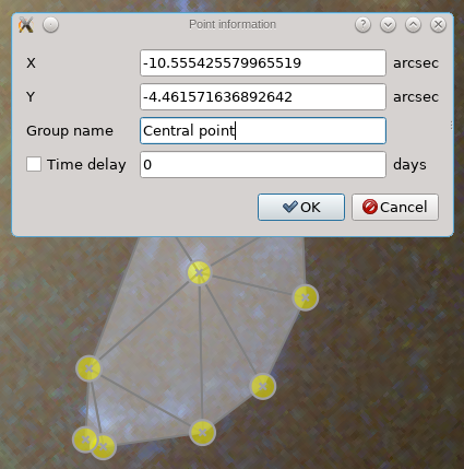
If you right-click on a point, a dialog is shown with various properties of that point; an example is shown below. You could change the coordinates somewhat if you like, provide a label/group name to the point, and possibly a time delay. In the current inversion procedure, the time delays are expected as a number of days.

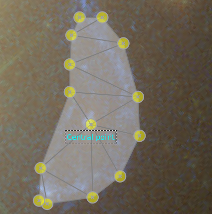
If you only want to provide a label/group name to a point, to indicate which points correspond to each other in different images, you can also just double click on a point that’s not selected (so a yellow point, not a blue one). You’ll then see a dotted rectangle in which you can type a label, as the figure below shows.

In the Edit menu, there’s an option called Create null grid, with which you can create null space grids for use in inversions with point images or extended images. For extended images, the inversion routine assumes a grid in which the regions where images are observed, or where extra images could be observed, are cut out. For inversions with point images, a very simple grid is typically used, there’s no need to cut out anything.

The tool is the same for both cases, and it will decide if regions need to be cut out based on the visible points layers. So if you want to create a simple null grid, without removing any regions, make sure that all points layers are hidden (using the checkbox next to the layer name). Assuming that this case is fairly straightforward, let’s focus on the case in which we do want to remove certain regions.

In the screenshot below, four extended images were drawn (very roughly, just for this example). In the editor, there are two main ways to specify different images. A very simple one, that is not used in the example below, is to have a points layer for each image. Another approach is to have several images in the same layer, but then triangulations are needed to be able to detect that there are in fact multiple images in that layer. If there are only points, there’s no way to automatically detect which points belong together in one image, but if triangulations are present then these can be used to figure out which points belong to which image.

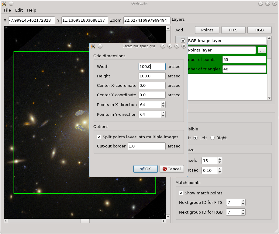
When the tool is started from the Edit menu, a dialog box appears, as you can see below. There you can specify the size of the grid, as well as its center, and the number of points in each direction, which determines how small or how large the triangles in between will be. It is usually a good idea to make the region considerably larger than the strong lensing region, to avoid the inversion routine getting fooled by extra, far away images that lie completely outside the null space region.

If no points layers are visible, then a regular grid would be the result, but if points layers are present, the images therein will be removed from the null space grid. It is usually a good idea to remove a slightly larger region than the images themselves, so that there’s no null space penalty anymore if the back-projected images don’t overlap perfectly (this is never the case). That’s what the Cut-out border option is for. If multiple images are present in the same points layer (see above), as is the case here, the Split points… option needs to be checked to detect them. If it is not checked, only a single image is assumed per layer, and if that image can’t be reconstructed from the triangulation info, then the convex hull of all points will be used as the image shape. In this example, unchecking that option would cause the entire region enclosed by the images to be removed from the null space grid.

When you’re satisfied with all the options, just press Ok and the null space grid is generated. A new points layer is automatically added, containing the generated points and the triangulation. For the example we’re considering, the result is shown below (the grid is larger than the current viewport though), and you can see that the image regions, as well as an extra border, have been removed from the null space. If you want to do this programmatically in a script, perhaps useful to create grids with the same settings for many multiple-image systems, you can use the createGridTriangles routine. Always check the resulting generated grids! You can show them either in the GRALE Editor, or using plotImagesData.

Exporting to and importing from ImagesData files

All info that you’re working with in the GRALE Editor, all layers and their settings, can be saved to a file, and loaded from a file, from within the File menu. This saves the information in a straightforward JSON format, which can be edited manually if needed, for example to change the path for one of the FITS or RGB files. The FITS or RGB data itself, the pixel values, are not stored in that file, only the file name paths. If you’d like to share such a saved JSON file with someone else, this means you’d have to share the FITS or RGB files separately. The receiver may need to adjust the paths to those files in the JSON file.

Ultimately, we’re interested in creating input for a lens inversion, which requires ImagesData instances for the images or null space. The Export to images data and Export options entries, both in the File menu as well, allow you to write the points layers to files which can later be loaded again as ImagesData objects in an inversion script.

The Export options entry, contains the following three items that control the export procedure:

• Split layer into images

• Export groups

• Export time delays

In any case, only points layers (note that a null space grid is also a points layer) can be stored into an ImagesData file, and only visible points layers are considered when exporting. If the first option, Split layer into images is not checked, then each visible points layer will be stored as a separate image in the ImagesData instance. When the option is checked, additionally each points layer will be split into several images based on the triangulation info (as explained before), potentially leading to more images than visible points layers. This is very useful when all images are simply stored in a single points layers.

The labels/group names you assign to points define which points inside extended images are actually point images of the same point source. Such point groups can be stored in an ImagesData file, and it’s likely that you want to leave this option checked to do so. If for some reason you’d like to forget about the group info, you can uncheck this.

While the points belonging together can be stored in this way, the names you assign to them, the labels, are not stored in an ImagesData instance. When you export to and later import from an ImagesData file, instead of the names you assigned to the points, you’ll only see numbers. The points in the same group will still have the same number of course.

The last option, Export time delays is quite self-explanatory. It merely controls if the time delay data that you’ve entered is written to the ImagesData file as well. Usually you’d want to leave this checked.

Note that for convenience these export options are remembered, so if you’re not sure what will be exported it may be a good idea to double check this. To actually export the file, you’d select the Export to images data option and specify a file name.

The Import images data option actually has two variants:

• Points layer per image

• All in one points layer

If the first option is selected, every image contained in the ImagesData file is introduced as a separate points layer. In the second case, all images from the file are added to a single points layer. Note that if the file does not contain triangulation information, it may be difficult to split the layer into separate images again. In both cases, new points layers are simply added to the current GRALE Editor scene, nothing will be overwritten or deleted.

Saving the view to an image file (PNG or JPG)

In the File menu, there’s an entry Export area/view; you can use this to save what’s currently shown to e.g. a PNG or JPG image. All visible layers are considered, using the current point sizes. In the dialog that is shown when you select this option, you can choose either to save the area that’s currently shown, or an area with the dimensions specified in the dialog. You can also specify the number of pixels in the resulting image.

This can come in handy to create an overlay of the reconstruction of the mass density on top of an observation. If the reconstruction whould show the mass density in a 30x30 arcsec region centered on the origin for example, this tool allows you to export the same region to an image, and load that again in a script to create a mass density plot overlayed on this background:

# Read the background image exported using the GRALE Editor
rgb = plt.imread("./a3827_background_30x30.png")

# Here we need to tell how the image pixels map onto the coordinate system:
# In the GRALE Editor, the RA axis pointed left, so the left most pixel is
# at 15 arcsec, the rightmost at -15 arcsec. The bottom pixel corresponds
# to a declination of -15 arcsec, the top pixel to 15 arcsec.
plt.imshow(rgb, extent=[15,-15,-15,15])

# Draw several contour levels
plotutil.plotDensityContours(lensInfo, densityUnit=critDens, levels=np.arange(0,10,0.2), cmap="gray")
# Redraw the critical density contour as a think white line
plotutil.plotDensityContours(lensInfo, densityUnit=critDens, levels=[1], linewidths=[3], colors="white")
# Show the RA axis pointing left instead of right
plt.gca().invert_xaxis()

This would then produce the following plot:

Back-projecting images using a lens model and re-lensing them

With the result from an inversion, you can use the GRALE Editor to backproject one or more image regions as currently displayed, e.g. from a FITS file or overlayed RGB file. These backprojected images will then be used as a source, and the lens effect will be recalculated. For example, suppose we’ve indicated one image in the viewport as follows:

In the Edit menu, there’s a tool called Back-project and retrace that in this case will determine the image region based on the points layer. It then hides the points layers themselves, and based on the visible FITS/RGB layers will grab what the image looks like. This all uses the FITS/RGB layers as displayed, it will not use the raw FITS values for example.

The simplest case uses only one image, and calculate the entire image plane in one go. The result of the tool is that two RGB layers are added to the scene: one containing the estimated source, so the back-projected image region, and one containing the re-lensed images. In this example, when hiding the re-lensed images, the resulting scene with the added source estimate, would look as follow:

If we hide this back-projected image, but show the re-lensed images based on the lens model and this source estimate, the result is shown below. This is shown on top of the existing layers, which is why you see the yellow dots from the points layer still peeking out from underneath.

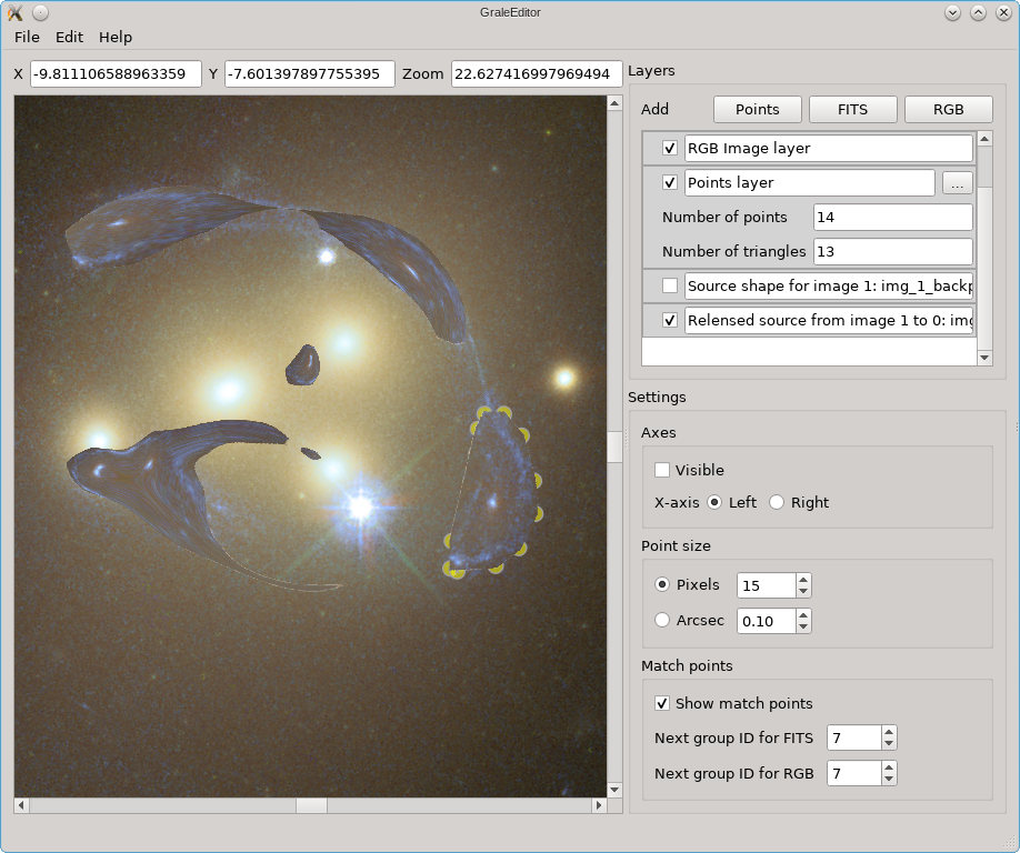
This represents one of the simplest uses of the tool. One step more complex is to use one or more points layers to indicate more than one image. Each image will then be considered separately, creating a back-projected version and re-lensing this. Depending on the detail that you like, instead of tracing the entire lens plane, you can also recalculate only the image regions that you indicated, based on each source estimate. As this limits the size of the regions that need to be calculated, allowing you to get a better resolution there, you won’t get results for the image plane that don’t have image shapes assigned to them in some points layer. In the example above, we’d still get that one source estimate, but we’d only recalculate the region that we indicated in the points layer. No estimates of the other images would be calculated in the re-lensing procedure.

When you start the tool from the Edit menu, you’ll see a dialog like the one below. Near the top, no image plane info will be shown however, you’ll need to load that first. To create such a file, you need to get an ImagePlane for the redshift of the source/images that you’re considering, and use pickle to create a file. This file should have the extension .dat or .imgplane for the tool to recognize it. You can create this ImagePlane manually by first creating a LensPlane from your lens model. An easier way may be to create a LensInfo instance first, and then to call its getImagePlane method, e.g:

li = plotutil.LensInfo(lens, size=50*ANGLE_ARCSEC, zd=zd, zs=zs)
imgPlane = li.getImagePlane()
pickle.dump(imgPlane, open("test.imgplane", "wb"))

When you click the Load button, you can load this file into the tool; you can specify an arbitrary description, that’s just for yourself to known which image plane has been loaded in case you need the tool again, perhaps for a source at another redshift (in which case you’d need to load another image plane file).

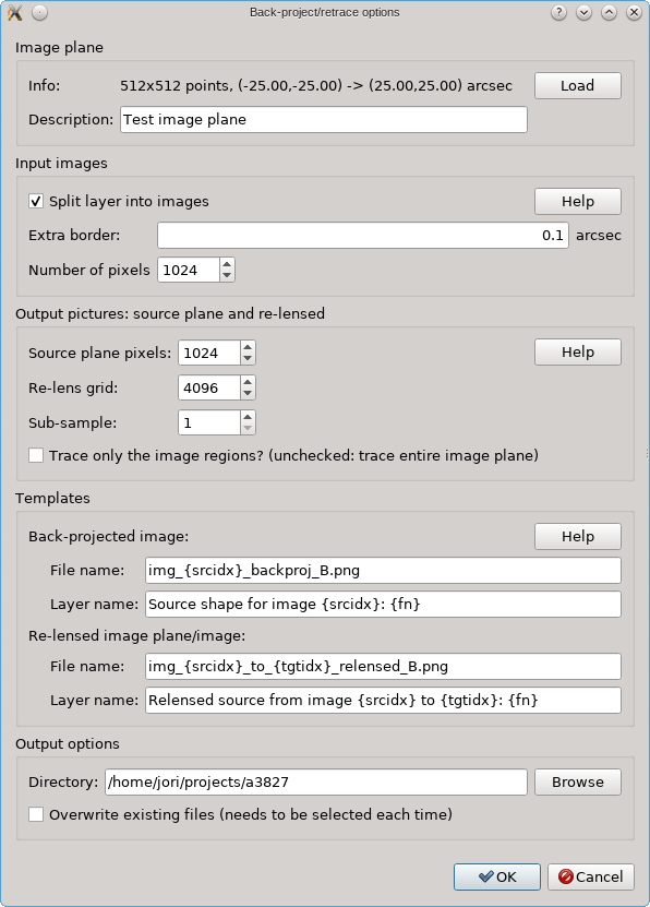
The various other options all have a Help button to explain what they mean. There are options to specify how the input regions should be constructed, and with what resolution they should be turned into pictures. The output has two modes as explained above: either the entire image plane is re-lensed, or only the image regions are re-calculated. When the tool is run, new PNG files are created which are shown in new RGB layers. The Templates control the layer names and file names. By default these files are not overwritten if they already exist, for safety reasons, but there’s an option to allow that. Care must be taken when not using new file names however: the RGB layers only store the names to these files, so if they are overwritten by a new run of the tool, a layer may suddenly refer to different contents which may only become available when the layer is re-loaded.

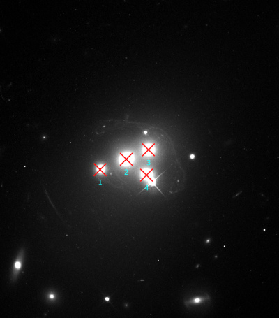
Looking for corresponding image points on back-projected images

The CL0024+17 cluster is a gravitational lens system containing a set of five extened images in which some corresponding points can easily be identified. In the scene below, a FITS image of this system was loaded in the editor, a points layer was added, and a very rough contour of the images was created by simply drawing the contour (as explained above).

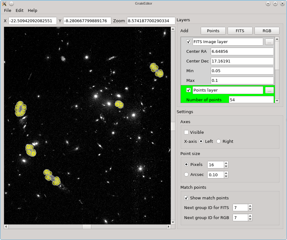
To help identify corresponding points in these extended images, it would be helpful if we could quickly change the view, focusing on each image in turn. This can be done using the Point select - no back-projection tool that can be accessed from the Edit menu. This first shows a dialog to control e.g. how the different images are identified; there’s a Help button to provide more information about the options. When you click Ok, the actual tool is started, and a window like the following is shown:

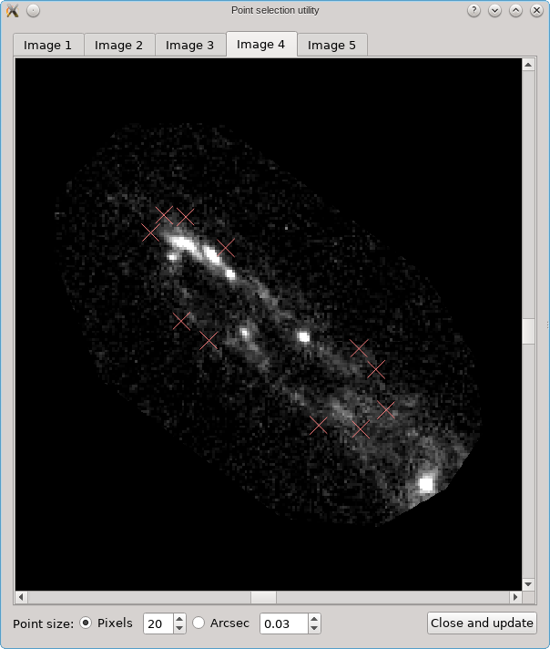
A similar background is shown as was visible in the main viewport of the editor, but only for the image region that was detected. Several tab pages are available, one for each of the images. The points that are relevant for each image are shown as well, and their size can be controlled by the options near the bottom, similarly as in the main editor.

Now, you can add or move points, and you can also provide labels to the points. This way, you can identify corresponding points in the different images. To add a label, you can first add a point using a left click, and then double click that point. You can also just keep Ctrl (or Cmd) pressed during the left click to add the point, which will immediately allow you to start typing. By switching from image to image, you can add several corresponding points, as is shown below:

When you click the Close and update button, the changes you’ve made (points added, moved, deleted, or labels changed) will be passed to the main editor. When you simply close the window, all changes will be lost however!

Note that if points were added, they will not automatically be inserted into a triangulation that may be present for an image. If you need this to be the case, you can simply select all points/triangles for that image (includes the new points), press Ctrl+Delete to delete only the triangles, and finally double click on one of the (selected) points to generate a new triangulation.

Depending on the situation, you could export the extended images, including the corresponding points, to an ImagesData file. Alternatively you could create input for a point image inversion, but that requires you to get the coordinates of the corresponding points only. Saving the extended images first to an ImagesData file and processing the point groups stored therein is one possibility. Alternatively you could directly analyze the JSON file (Python has a json module) that you get when you save the scene in the editor.

While being able to switch from image to image can certainly help to identify corresponding features, the fact that the gravitational lens distorts each image, flipping it and stretching it in various ways, makes the identification somewhat less straightforward. In case you have a model for the lens at hand, perhaps from a first rough identification of corresponding points, you can use this to back-project these image regions first, and look for corresponding points in the back-projected images.

This is done using the tool Point select - back-project first, also in the Edit menu. The dialog that’s shown allows you to load an image plane file, similar as in the back-project/re-lens tool that was discussed previously. Other options again have a Help button for more information, and are similar as in the point select tool without back-projecting first.

After the dialog, a similar window is shown as before. The main difference is that the image regions have been projected back onto their source planes, and that for each back-projected image, the same source plane region is always shown. This means that if you zoom in one of the tabs, you’ll also zoom in the other tabs. Having a lens model may make it much easier to identify corresponding points, and you can end up with back-projected images that match quite well:

If you add or move points, when you click the Close and update button, their corresponding location in the image plane is calculated using the information about the lens model that was loaded.

So far in the example, we’ve only used a FITS layer to get the shape of the images. If you have an RGB version of the same region at hand, or if you can make one based on several FITS files, it can be much easier to identify the points. Since the tool always shows the same region in the source plane, but for different images, it can easily be used to get an idea about how well the back-projected images (so the source estimates) overlap. In the animation below, the point size was set to 0 to hide the points and only shown the back-projected images:

Pro-tips

The command line

On the command line, you can specify a previously saved JSON file as the first argument, causing this file to be loaded. With other file names you can add to this scene: for example if another JSON file is specified, its layers will be added to the existing ones. You can add layers from other files as well, and you don’t need to specify a JSON file first for this to work.

If a JPG, PNG or FITS file is specified the corresponding layer will be added. Note that in this case, no alignment or recentering will be done in advance as there isn’t any available data yet. Specifying a . on the command line adds a new points layer to the scene. With myimagesfile.imgdata or N,myimagesfile.imgdata you can add one or more points layers with information from the specified file. In the first case, all points from all images in the file will be added to the same points layer, including the triangulations if present. In the second case, if N is zero or more, it specifies a specific image in the file (counting starts with 0) that should be imported into a new points layer. In case N is negative, all images will be imported again, but each in its own points layer.

When exiting the GRALE Editor, it should give you a warning if there are unsaved changes. For some workflows this could cause unnecessary delays, and to prevent this dialog from interfering you can specify --nocheck on the command line. We will see an example of this below. In that example we’ll also encounter the option --imgdataname:myexportfile.imgdata to set the file name that will be proposed when exporting the points layers to an ImagesData file.

For completeness, with --imgplane:myimgplane.dat you can pre-load a pickled image plane for use with the tools that require backprojecting the images, and with --zoom:X you can set the zoom factor to a specific value.

Shortcut keys

If a point is selected, pressing c centers the view on that point. When exporting to an ImagesData file and you’ve selected that individual images should be determined from the triangulation info, it’s possible that this fails, for example perhaps you’ve unknowingly added added a point by a mouse click. If this fails, you’ll be asked if you’d like to select the point that triggered the failure. Since this may be difficult to spot, perhaps it’s outside the current view for example, centering on the point may be helpful.

By pressing 1 … 9, you automatically set the zoom level to 2 ^N, depending on the pressed key (actually 0 also works). This can also help in the previous scenario: just centering on the point may not be clear enough depending on the number of points in the neighbourhood and the zoom level. By changing the zoom without changing the location in the center, the point can more easily be identified.

If Ctrl (or Cmd on OS X) is pressed at the same time one of the 1 … 9 keys is pressed, the editor will look for the corresponding points layer, make it active, and center on it. This will only be helpful if each image is present in its own points layer, for example by specifying -1,myfile.imgdata on the command line. If Ctrl-1 is pressed, the first points layer will be used, Ctrl-2 uses the second points layer, etc.

Above, it was explained how the contour finder tool can be started by having a points layer active, and double clicking on a point in the background FITS layer for example. Instead of double clicking, you can also press Ctrl-L (or Cmd-L on OS X), in which case the position that’s currently centered on will be used.

As is often the case, pressing Ctrl-S (Cmd-S on OS X) is a shortcut for saving the entire scene, to a JSON file in case of the GRALE Editor. There’s also a shortcut to export the visible points layers to an ImagesData file: Ctrl-E (or Cmd-E on OS X). This is the same as selecting the entry from the menu, so the same export options will be used.

Example workflow: extended images from point images

TODO:

• point images to imgdata files

• actions for one imgdata file

• bash loop all image files